Chapter II
From Deep Learning to Deep Voting
Chapter Summary
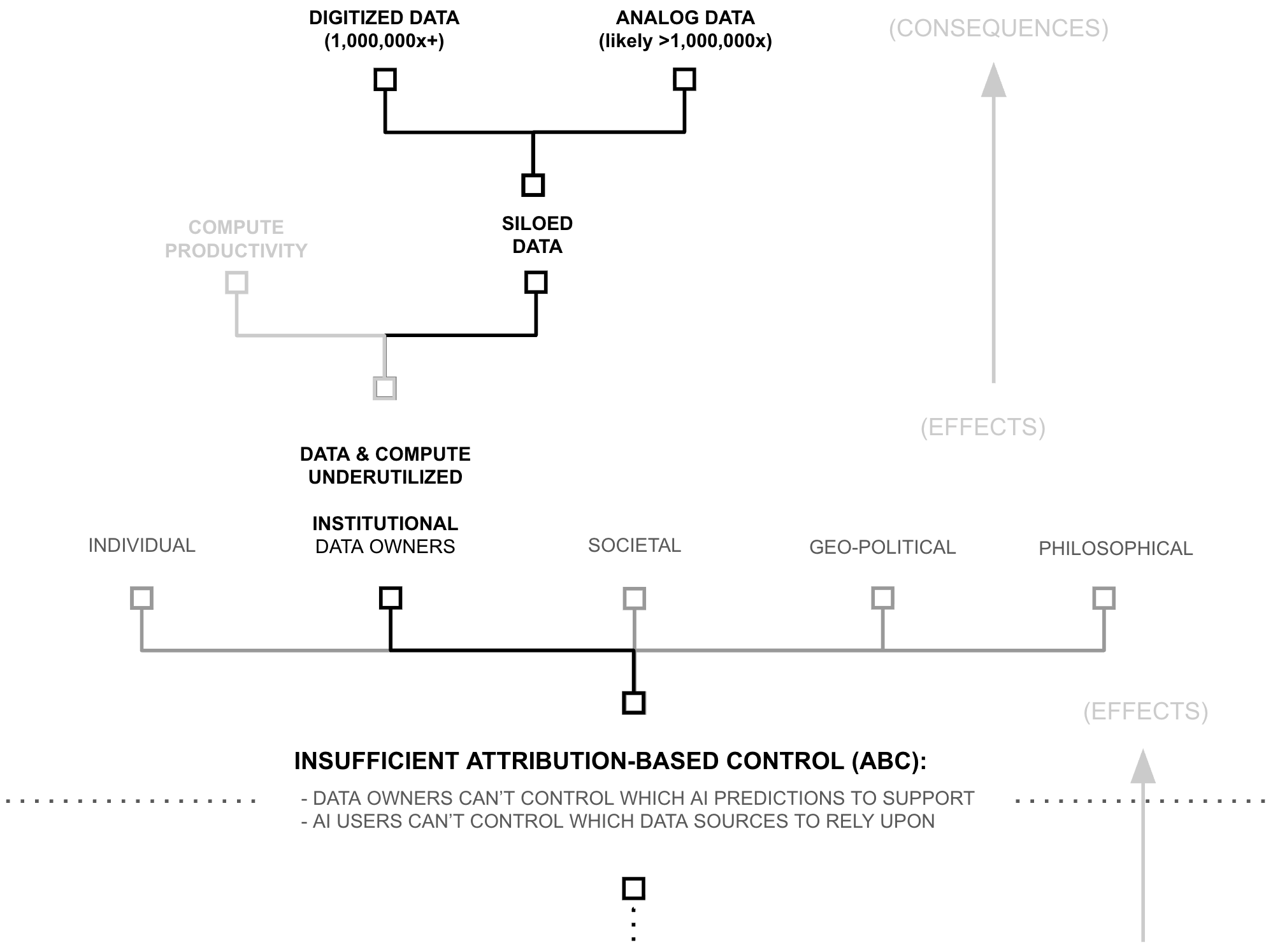
Estimates below suggest that models are trained using less than 1/1,000,000th of the world’s data and AI compute productivity. Consequently, following AI’s scaling laws (Kaplan et al., 2020; Hoffmann et al., 2022), AI models possess capabilities which are insignificant compared to what existing data, compute, and algorithms could create.
Yet, if AI models (and their capabilities) are the lifeblood of the AI industry, why are data and compute so underutilized? Why is AI capability so constrained? This chapter unpacks the cause of such a drastic resource under-utilization. It begins by linking resource utilization to attribution-based control (ABC). It then breaks attribution-based control into problems with attribution and control, which are themselves underpinned by deep learning’s core philosophy of mixing dense features. This mixing is only problematic because of a specific technical choice: the use of addition to update model weights, which erases provenance information during gradient descent.
The chapter then explores alternatives to addition during the training process, revealing a fundamental trade off between three factors: AI capability (driven by unrestricted feature learning), attribution (tracking where features came from), and computational complexity (tracking the path of feature mixing). It proposes a key innovation, a re-purposing of differential privacy for attribution: differential attribution, using the natural boundaries of training documents to identify which concepts must mix freely and vice versa, thereby pushing this Pareto frontier by providing a data-driven approach to balance addition and concatenation.
Building on this insight, the chapter develops a specific form of concatenation to replace addition in key sections of the deep learning training process. This transformation—from deep learning to deep voting—cascades upward through the aformentioned hierarchy of problems, reducing the need for dense feature mixing across data sources, enabling attribution-based control, and unlocking a viable path towards another 6+ orders of magnitude of training data and compute productivity. Taken together, the chapter reveals how a seemingly technical choice (the use of addition) creates far-reaching consequences for AI systems, and how careful, data-driven use of concatenation may dramatically expand AI’s access to computational and data resources.
The Symptom: Data/Compute Underutilization
As of NeurIPS 2024, leading AI researchers have reported that available compute and data reserves are approaching saturation, creating constraints on both computational resources and pre-training scale (Robison 2024; Strati et al., 2024). However, this assessment overlooks approximately six orders of magnitude of underutilized compute productivity and siloed data. Rather than absolute scarcity, the industry faces structural problems of data and compute access and productivity.
6+ OOM: Underutilized Training Compute Productivity
The AI industry’s computational requirements have driven significant economic and geopolitical consequences, including NVIDIA’s rise to become the world’s most valuable company, U.S. export restrictions on AI chips to China, and intense competition for latest-generation hardware among startups, enterprises, and major technology firms (Kaye 2025; Kachwala and Bajwa 2025; Howley 2023). However, recent evidence suggests that current AI training and inference processes utilize less than 0.0002% of available compute productivity, indicating that perceived compute scarcity may reflect inefficiency rather than absolute resource limits. To evaluate this claim, this section estimates computational waste in two key activities: inference (forward propagation) and learning (backpropagation and gradient descent).
2-3 OOM: Inefficient AI inference
Due to its role in commercial deployments, analysts estimate that AI firms spend billions of dollars annually on inference (You 2025). However, while these costs might appear to reflect fundamental requirements for achieving high performance, a growing body of empirical work indicates substantial inefficiency in current inference practices.
A Library Analogy
Consider a library. When someone asks a librarian about the rules of chess, the librarian doesn’t subsequently read every book in the library to find the answer. Instead, they use the catalog system to find a relevant bookshelf, the titles of books on that shelf to find the relevant book, and the table of contents of that book to find the relevant section. This practice stands in stark contrast to how AI systems process information. To make an AI prediction with a model like GPT-3, AI users forward propagate through the entire model and all of its knowledge (i.e., read every book in the library). And in the case of large language models, they don’t just do this once per answer, they do this for every token they predict. This is analogous to a librarian reading every book in the library every time they utter a word. Given how implausible it is that any prediction requires the entirety of an AI models knowledge, AI’s full, dense inference is a staggering inefficiency.
AI models store information within their weights. General-purpose models (e.g., Gemini, ChatGPT, Claude, Llama) encode substantial portions of their training corpora (often representing significant fractions of publicly available internet data) in these parameters. However, when models like GPT-3 generate predictions, they forward propagate through every non-embedding parameter in the network, regardless of query relevance. This constitutes a form of exhaustive computation wherein all stored knowledge is activated for each inference, analogous to searching an entire corpus rather than querying relevant subsets.
From an information-theoretic perspective, this practice is inefficient; the relevant question concerns the magnitude of this inefficiency. A comprehensive answer would require empirically measuring the maximum percentage of model weights that can be excluded from inference without degrading accuracy. While such systematic measurement remains incomplete, existing work provides lower bounds on potential efficiency gains.
DeepMind’s RETRO achieves comparable performance to GPT-3 while using 1/25th of the parameters through retrieval from a large-scale vector database (Borgeaud et al., 2022). Similarly, Meta’s ATLAS demonstrates that models can be reduced to 1/50th their original size while maintaining or exceeding baseline performance through database-augmented inference (Izacard et al., 2023).
We adopt RETRO/ATLAS-style parameter efficiency as a conservative lower bound on current compute waste, noting that these approaches have not been widely adopted in either the sparsity literature (Lederer 2024) or frontier AI deployments, nor have comparable efficiency gains been demonstrated through alternative methods (cf. the persistent redundancy problem in Mixture of Experts models (Dai et al., 2024)). These results suggest that at least 96-98% of parameters activated during dense inference are unnecessary for individual queries.
This estimate is likely conservative, as it implies that 2-4% of a model’s knowledge base is relevant to any individual query. 1 However, parameter overuse during forward propagation represents only one source of computational waste. A second form of inefficiency arises in how models store and access information.
A Library Analogy
Consider a library once again. When someone asks a librarian about the rules of chess, and the librarian goes to fetch a particular book, the librarian doesn’t bring back every copy of the book in the library. And, as unintuitive as this might seem, the librarian also doesn’t bring back empty books from random assortments of shelves. Instead, they use the catalog system to find a relevant bookshelf, the titles of books on that shelf to find the relevant book, and then they select a single book for the library’s customer.
This practice stands in stark contrast to how AI systems process information. To make an AI prediction within a model like GPT-3, AI users don’t merely forward propagate through the entire model and all of its knowledge (i.e., read every book in the library), AI users must forward propagate through some mixture of multiple copies of the same information (i.e. multiple copies of the same book) as well as empty vector space (i.e. empty books) in order to create an output.
1 While this fraction seems implausibly large for most queries, systematic measurement of query-specific parameter relevance remains limited in the literature. We therefore retain this conservative 2-4% estimate.
Recent work demonstrates that current architectures contain redundant and underutilized parameters. Guo et al. achieve 5-10x reduction in parameter count through lossless compression while maintaining accuracy: ”Notably, we distill CIFAR-10 and CIFAR-100 to 1/5 and Tiny ImageNet to 1/10 of their original sizes without any performance loss on ConvNet, offering the first lossless method of dataset distillation” (Guo et al., 2023). This compression has been demonstrated across multiple standard architectures, as shown in Table 2.1.
| Dataset | CIFAR-10 | CIFAR-100 | Tiny ImageNet | |||||||||
|---|---|---|---|---|---|---|---|---|---|---|---|---|
| IPC | 1 0.02 |
10 0.2 |
50 1 |
500 10 |
1000 20 |
1 0.2 |
10 2 |
50 10 |
100 20 |
1 0.2 |
10 2 |
50 10 |
| Random | 15.4±0.3 | 31.0±0.5 | 50.6±0.3 | 73.2±0.3 | 78.4±0.2 | 4.2±0.3 | 14.6±0.5 | 33.4±0.4 | 42.8±0.3 | 1.4±0.1 | 5.0±0.2 | 15.0±0.4 |
| DC | 28.3±0.5 | 44.9±0.5 | 53.9±0.5 | 72.1±0.4 | 76.6±0.3 | 12.8±0.3 | 25.2±0.3 | - | - | - | - | - |
| DM | 26.0±0.8 | 48.9±0.6 | 63.0±0.4 | 75.1±0.3 | 78.8±0.1 | 11.4±0.3 | 29.7±0.3 | 43.6±0.4 | - | 3.9±0.2 | 12.9±0.4 | 24.1±0.3 |
| DSA | 28.8±0.7 | 52.1±0.5 | 60.6±0.5 | 73.6±0.3 | 78.7±0.3 | 13.9±0.3 | 32.3±0.3 | 42.8±0.4 | - | - | - | - |
| CAFE | 30.3±1.1 | 46.3±0.6 | 55.5±0.6 | - | - | 12.9±0.3 | 27.8±0.3 | 37.9±0.3 | - | - | - | - |
| KIP1 | 49.9±0.2 | 62.7±0.3 | 68.6±0.2 | - | - | 15.7±0.2 | 28.3±0.1 | 37.9±0.3 | - | - | - | - |
| FRePo1 | 46.8±0.7 | 65.5±0.4 | 71.7±0.2 | - | - | 28.7±0.1 | 42.5±0.2 | 44.3±0.2 | - | 15.4±0.3 | 25.4±0.2 | - |
| RCIG1 | 53.9±1.0 | 69.1±0.4 | 73.5±0.3 | - | - | 39.3±0.4 | 44.1±0.4 | 46.7±0.3 | - | 25.6±0.3 | 29.4±0.2 | - |
| MTT2 | 46.2±0.8 | 65.4±0.7 | 71.6±0.2 |
|
|
24.3±0.3 | 39.7±0.4 | 47.7±0.2 | 49.2±0.4 | 8.8±0.3 | 23.2±0.2 | 28.0±0.3 |
| TESLA2 | 48.5±0.8 | 66.4±0.8 | 72.6±0.7 |
|
|
24.8±0.4 | 41.7±0.3 | 47.9±0.3 | 49.2±0.4 | - | - | - |
| FTD2,3 | 46.0±0.4 | 65.3±0.4 | 73.2±0.2 |
|
|
24.4±0.4 | 42.5±0.2 | 48.5±0.3 | 49.7±0.4 | 10.5±0.2 | 23.4±0.3 | 28.2±0.4 |
| DATM (Ours) | 46.9±0.5 | 66.8±0.2 | 76.1±0.3 | 83.5±0.2 | 85.5±0.4 | 27.9±0.2 | 47.2±0.4 | 55.0±0.2 | 57.5±0.2 | 17.1±0.3 | 31.1±0.3 | 39.7±0.3 |
| Full Dataset | 84.8±0.1 | 56.2±0.3 | 37.6±0.4 | |||||||||
Because they account for information waste in different ways, these inefficiencies compound multiplicatively: irrelevant parameters (25-50x+) and redundant parameters (5-10x+) suggest a 125-500x+ lower-bound to inference inefficiency. And while these are estimates, both bounds come from working implementations that maintain model performance, using techniques which are not widely popular, suggesting this waste is common in frontier AI systems, and that this waste stems from architectural choices rather than fundamental limitations
6 OOM: Underutilized and Inefficient Compute in AI Learning
AI firms famously spend immense amounts of money training their AI models, a point which features heavily in their marketing (Meta AI 2024; Brown et al., 2020; Wiggers 2024). However, despite widespread hype around AI training spend, a theoretical inefficiency is backed by an increasingly large body of empirical observations, suggesting that the compute requirements for training AI models are largely misunderstood. To introduce the theory, consider an analogy.
A Library Analogy
As before, consider a library. When a library adds or removes a significant number of books to/from their collection, they don’t rebuild the entire building and re-print all of their books from scratch, they simply add/remove books, shelves, or rooms. These practices stand in stark contrast to how AI systems process information. To add or remove a significant portion of knowledge from a deep learning system, AI researchers retrain them from scratch (i.e., tear down the entire library, burn all the books, rebuild the library, and re-print all the books from scratch). Despite being a widespread, even ubiquitous practice within AI research, this practice is staggeringly inefficient. It re-characterizes the claims of compute scarcity in an entirely new light. It is like a librarian who repeatedly tears down their library, and re-prints all their books — lamenting insufficient bricks, paper, or ink.
AI models store information within their weights. To acquire this information, models are trained on large corpora at substantial computational cost (e.g., significant portions of the public internet) (Epoch AI 2025). However, when models require substantial updates (either incorporating new information or removing outdated content) current practice involves retraining from scratch (Goodfellow et al., 2016). This approach discards all previously computed parameters and repeats the entire training process, even when the majority of learned representations remain valid.
From an information-theoretic perspective, this practice is inefficient; the question concerns its magnitude. Comprehensive quantification would require detailed documentation of compute allocation within leading AI firms, information that is not publicly available. However, public disclosures and industry analysis provide sufficient data to establish lower bounds on this inefficiency.
Analysis of the largest AI firms reveals that pre-training their most capable models consumes less than 1% of quarterly compute budgets (see Table 2.2; methodology detailed in Appendices I and II). Yet these same firms continue expanding computational infrastructure to support larger models (Mehta 2024; OpenAI 2024; Sevilla and Roldan 2024), suggesting that remaining compute capacity is allocated to other training activities rather than final model production.
| Model | Organization | Lab/Cloud | Train FLOPs |
Parent Org Peak Annual FLOPs |
Model/Public Models (Lab/Cloud) |
Model/Peak Annual (%) |
Model/Peak w/100x (%) |
|---|---|---|---|---|---|---|---|
| Gemini 1.0 Ultra | Google DeepMind | Google DeepMind | $5.00 \times 10^{25}$ | $3.87 \times 10^{28}$ | 45.65 | 0.129 | 12.93 |
| Claude 3.5 Sonnet | Anthropic | Anthropic/Amazon | $4.98 \times 10^{25}$ | $2.27 \times 10^{28}$ | 69.74 | 0.220 | 21.96 |
| GPT-4o | OpenAI | Microsoft/OpenAI | $3.81 \times 10^{25}$ | $4.35 \times 10^{28}$ | 53.36 | 0.088 | 8.75 |
| Llama 3.1-405B | Meta AI | Meta AI | $3.80 \times 10^{25}$ | $5.65 \times 10^{28}$ | 66.32 | 0.067 | 6.72 |
| GPT-4 | OpenAI | Microsoft/OpenAI | $2.10 \times 10^{25}$ | $4.35 \times 10^{28}$ | 29.41 | 0.048 | 4.82 |
| Gemini 1.0 Pro | Google DeepMind | Google DeepMind | $1.83 \times 10^{25}$ | $3.87 \times 10^{28}$ | 16.71 | 0.047 | 4.73 |
| Claude 3 Opus | Anthropic | Anthropic/Amazon | $1.64 \times 10^{25}$ | $2.27 \times 10^{28}$ | 22.97 | 0.072 | 7.23 |
| Gemini 1.5 Pro | Google DeepMind | Google DeepMind | $1.58 \times 10^{25}$ | $3.87 \times 10^{28}$ | 14.43 | 0.041 | 4.09 |
| Llama 3-70B | Meta AI | Meta AI | $7.86 \times 10^{24}$ | $5.65 \times 10^{28}$ | 13.72 | 0.014 | 1.39 |
| GPT-4o mini | OpenAI | Microsoft/OpenAI | $7.36 \times 10^{24}$ | $4.35 \times 10^{28}$ | 10.31 | 0.017 | 1.69 |
| PaLM 2 | Google DeepMind | $7.34 \times 10^{24}$ | $3.87 \times 10^{28}$ | 6.70 | 0.019 | 1.90 | |
| Llama 3.3 | Meta AI | Meta AI | $6.86 \times 10^{24}$ | $5.65 \times 10^{28}$ | 11.98 | 0.012 | 1.21 |
| Amazon Nova Pro | Amazon | Anthropic/Amazon | $6.00 \times 10^{24}$ | $2.27 \times 10^{28}$ | 8.40 | 0.026 | 2.65 |
| Amazon Titan | Amazon | Anthropic/Amazon | $4.80 \times 10^{24}$ | $2.27 \times 10^{28}$ | 6.72 | 0.021 | 2.12 |
| Claude 2 | Anthropic | Anthropic/Amazon | $3.87 \times 10^{24}$ | $2.27 \times 10^{28}$ | 5.41 | 0.017 | 1.70 |
| Minerva (540B) | Google DeepMind | $2.74 \times 10^{24}$ | $3.87 \times 10^{28}$ | 2.50 | 0.007 | 0.71 | |
| GPT-3.5 (text-davinci-003) | OpenAI | Microsoft/OpenAI | $2.58 \times 10^{24}$ | $4.35 \times 10^{28}$ | 3.61 | 0.006 | 0.59 |
| U-PaLM (540B) | Google DeepMind | $2.53 \times 10^{24}$ | $3.87 \times 10^{28}$ | 2.31 | 0.007 | 0.65 | |
| PaLM (540B) | Google Research | Google DeepMind | $2.53 \times 10^{24}$ | $3.87 \times 10^{28}$ | 2.31 | 0.007 | 0.65 |
| Flan-PaLM 540B | Google DeepMind | $2.50 \times 10^{24}$ | $3.87 \times 10^{28}$ | 2.28 | 0.006 | 0.65 | |
| FLAN 137B | Google Research | Google DeepMind | $2.05 \times 10^{24}$ | $3.87 \times 10^{28}$ | 1.87 | 0.005 | 0.53 |
| Meta Movie Gen Video | Meta AI | Meta AI | $2.65 \times 10^{24}$ | $5.65 \times 10^{28}$ | 2.88 | 0.003 | 0.29 |
| Megatron-Turing NLG 530B | Microsoft,NVIDIA | Microsoft/OpenAI | $1.17 \times 10^{24}$ | $4.35 \times 10^{28}$ | 1.64 | 0.003 | 0.27 |
| Llama 2-70B | Meta AI | Meta AI | $8.10 \times 10^{23}$ | $5.65 \times 10^{28}$ | 1.41 | 0.001 | 0.14 |
The contrast between frontier models consuming a small fraction of quarterly compute budgets and ongoing infrastructure expansion suggests that leading AI firms train numerous experimental models beyond their final deployments. This interpretation aligns with widely documented practices in frontier AI laboratories. Major labs employ hundreds to thousands of researchers who routinely train models during development. Standard optimization procedures, such as hyperparameter sweeps, involve training single model architectures tens to hundreds of times to identify optimal configurations (Weights & Biases 2025).
Taken together, producing a final frontier model requires training hundreds to thousands of intermediate models during the R&D process. While hyperparameter optimization is essential to model development, current approaches necessarily involve complete retraining for each configuration. This contrasts with modular systems where components can be incrementally optimized without discarding the entire structure. Recent work on targeted model modification (e.g., LLM surgery (Veldanda et al., 2024)) suggests alternatives to full retraining, but such techniques have not been widely adopted in frontier model development, necessitating substantial computational expenditure during optimization.
Consider the magnitude of this inefficiency. If frontier labs aim to produce general-purpose models, then computational resources allocated to intermediate experimental models represent overhead that does not directly contribute to final model capability. Based on Table 2.2, approximately 98.53% of annual training budgets are allocated to models other than the final deployment (calculated as 100% − (0.22%/15%), where 15% represents the estimated fraction of total compute dedicated to training (Bratt 2025)). Under the objective of producing a generalpurpose model, this implies that the vast majority of training compute is allocated to parameters that are ultimately discarded during the optimization process.
This annual estimate may understate total inefficiency, as it assumes frontier labs must train at least one model from scratch annually. If model parameters could be efficiently reused across generations (as RETRO/ATLAS demonstrate through their retrieval databases, where up to 98% of knowledge can be transferred between model versions (Borgeaud et al., 2022; Izacard et al., 2023)) the efficiency gap would be larger. However, retraining overhead represents only one source of computational waste. A second source arises from how models process information during training. To observe the theory behind this phenomena, consider the following analogy.
A Library Analogy
Once again, consider a library. When someone submits a new book to a library, the librarian doesn’t subsequently read every book in the library to figure out where to store it on the shelves. Instead, they use the catalog system to find a relevant bookshelf, the decimal system to locate the right placement on the shelf, and (perhaps) the title of the book to find its alphabetical placement on that shelf.
This practice stands in stark contrast to how AI systems are trained. To add a single training example into a model like GPT-3, AI users forward propagate through the entire model and all of its knowledge (i.e., read every book in the library). And to train an entire model like GPT-3 on modern training corpuses (i.e. trillions of tokens), it repeats this process trillions of times. It is like a librarian who repeatedly reads every book to figure out where a book should be placed, and then complains about not having enough librarian assistants (i.e. GPU compute threads) to accomplish the task.
The question concerns the magnitude of this inefficiency. The RETRO and ATLAS results previously discussed demonstrate that models can achieve comparable performance while being 25-50x smaller in parameter count. This parameter reduction translates directly to reduced training costs: fewer parameters require proportionally fewer FLOPs during both forward and backward propagation. The compression results further indicate that models can be trained with 5-10x fewer parameters without performance degradation, compounding the potential efficiency gains.
Yet, these three sources of training inefficiency (retraining overhead, dense forward propagation, and parameter redundancy) do not exhaust the potential efficiency gains. A fourth source arises from how models organize information during the training process itself.
A Library Analogy
Consider a brand new library. When a librarian goes to stock their library, they do not necessarily store every book in the universe in their library. Instead, libraries participate as a part of a library network. In this way, a nation-wide (or even global) community of libraries each store a cache of books, and when one user asks their local library for a book they do not have, that library will call in that book from another library. Through this process, even tiny, rural libraries are (in a way) making a massive, global collection of knowledge available to their local community. Some might even say that a small, local library makes all of humanity’s knowledge available to their local community, even if their local collection is small.
This practice stands in stark contrast to how AI systems are trained. Firms around the world are scraping the internet (or downloading web scrapes) and training their own models from scratch largely on the same information scraped from the internet. In these practices, they are encoding the same information redundantly across many organizations instead of building upon the existing knowledge already encoded into neural weights by other parties. That is to say, AI companies repeat each others’ work to a great degree.
AI models store information within their weights. General-purpose models encode substantial portions of publicly available internet data through training on large, overlapping corpora. Multiple organizations train models on similar or identical datasets, often drawn from common sources such as web scrapes and public repositories. This results in redundant encoding of the same information across independently trained models.
| Category | Computing Power (FLOP/s) |
Share (%) | Source/Calculation |
|---|---|---|---|
| Cloud/AI Providers | |||
| Meta | $1.79 \times 10^{21}$ | 5.57 | From Table 6.3 Total Q4 2024 |
| Microsoft/OpenAI | $1.38 \times 10^{21}$ | 4.29 | From Table 6.3 Total Q4 2024 |
| Google/DeepMind | $1.23 \times 10^{21}$ | 3.81 | From Table 6.3 Total Q4 2024 |
| Amazon/Anthropic | $7.19 \times 10^{20}$ | 2.23 | From Table 6.3 Total Q4 2024 |
| Consumer Computing | |||
| Smartphones | $7.48 \times 10^{21}$ | 23.23 | Sum of Active iPhones/Androids from Table 6.5 |
| PC CPUs/GPUs | $2.23 \times 10^{21}$ | 6.92 | Sum of PC CPUs and GPUs from Table 6.5 |
| Game Consoles | $8.64 \times 10^{20}$ | 2.68 | From Table 6.5 |
| Other Cloud/Pre-2023 | $1.65 \times 10^{22}$ | 51.28 | (see appendix for details) |
| Total | $3.22 \times 10^{22}$ | 100.00 | Sum of all rows above |
From an information-theoretic perspective, this redundancy is inefficient; the question is: how much? Comprehensive measurement would require documenting the overlap in training data and model capabilities across organizations, information that is not systematically available.
However, industry analysis provides order-of-magnitude estimates of aggregate underutilization. The largest AI firm controls less than 5.57% of global computing capacity (Table 2.3). If training resources could be pooled across organizations (analogous to libraries participating in a global network rather than maintaining independent collections) available compute would increase by a factor of approximately 100/5.57 ≈ 17.95x relative to any single firm’s capacity. This represents the theoretical gain from distributed training architectures that enable collaborative model development across organizational boundaries.
Yet, even these four training inefficiencies may not fully describe the inefficiency present in modern AI. To observe the theory behind this next problem, consider the following analogy.
A Library Analogy
Consider a brand new library which doesn’t even have any books in it yet. Let’s say the librarian is in a hurry, and so they take the first book, pick one of the empty shelves, set the book on that shelf, and then run to get the second book. Then, looking at the second book, they ask, ”is this similar to the first book... or different”. And if it’s similar to the first book, they put it closer to the first book on the shelves, and if it’s different from the first book, they put it farther away. This librarian repeats this process over and over until they encounter a problem. After 10,000 books (out of the millions they have to load), one of the bookshelves is full. So, because the shelf they need is full, they run to the next shelf and empty it... throwing books onto the floor to make space for their new book, which needs to be in this location. But now, they need to re-stock the books they just threw on the floor! They then pick up the books from the floor and attempt to find them all new places in the library, accidentally filling up shelves in the process. They then repeat this process many, many times... stocking and re-stocking all the books until a sensible organization emerges.
Or consider another librarian, who is opening a new library. But before they begin stocking books, they set up a Dewey Decimal System. They label each book in the system, count the number of books in each category, and plan their shelf capacity appropriately. Then, they take each book and load it into its appropriate shelf in a single pass. This second technique stands in stark contrast to how AI systems are trained. To add the first training example into an untrained model like GPT-3, AI users forward propagate through the entire model and all of its knowledge and store that information in random locations throughout the model. Then, as more training examples pile into the model, the model experiences catastrophic forgetting (Kirkpatrick et al., 2017) as collisions occur. And to train an entire model like GPT-3 on modern training corpuses (i.e. trillions of tokens), it repeats this process trillions of times.
Quantifying the computational cost of catastrophic forgetting remains challenging due to limited empirical work on information segmentation during training. RETRO and ATLAS provide partial evidence, as does work on curriculum learning and knowledge distillation. Kemker et al. observe that avoiding catastrophic forgetting requires approximately 40x larger model capacity (Kemker et al., 2018), though this estimate is not especially recent. Multiple sources of training inefficiency compound: full model retraining during updates, dense forward propagation through all parameters, parameter redundancy from insufficient compression, and capacity overhead to prevent catastrophic forgetting during sequential training.
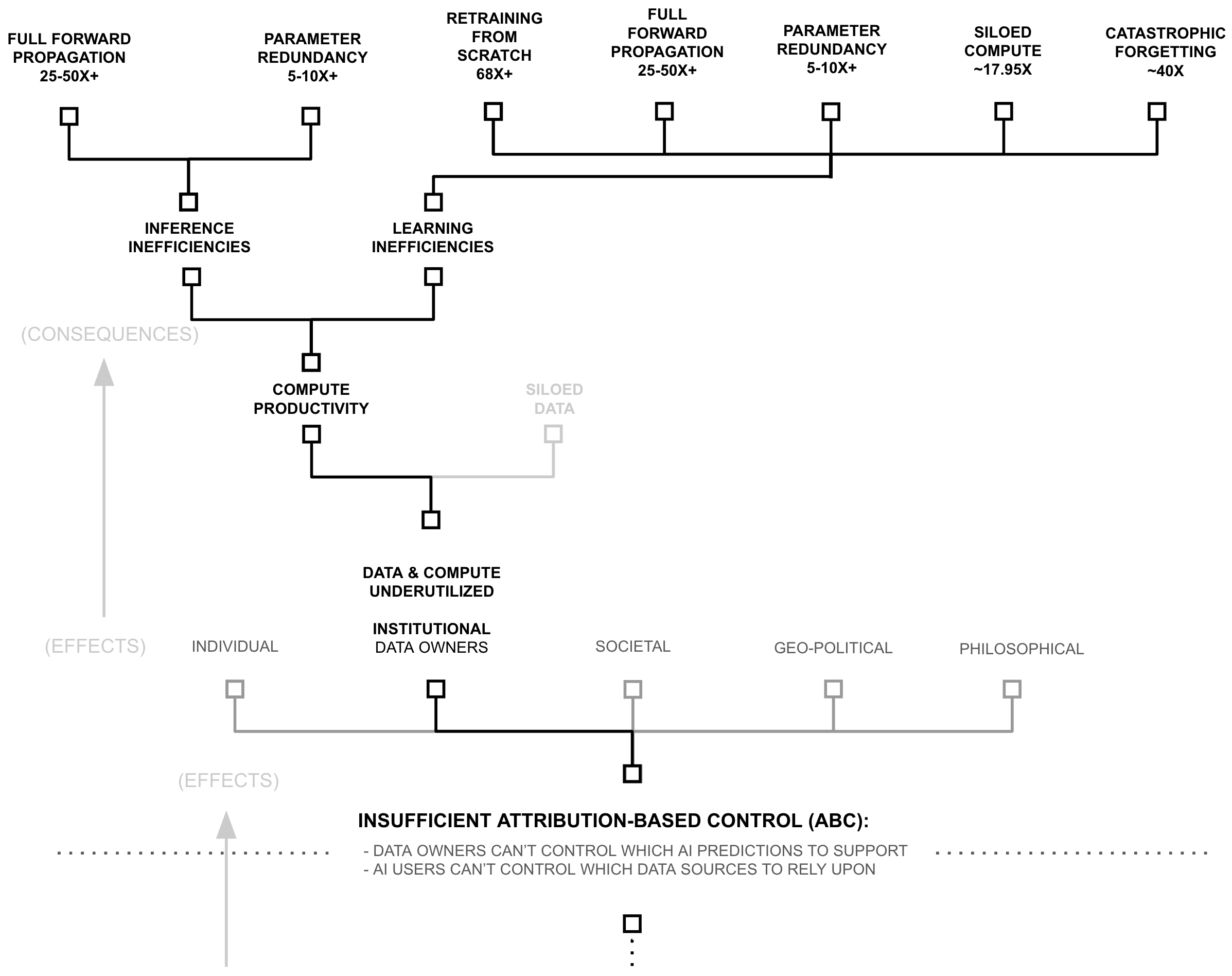
These inefficiencies compound multiplicatively in terms of FLOPs. Parameter reuse across model generations could increase compute productivity by a factor of 100/(100 − 98.53%) ≈ 68x. RETRO/ATLAS-demonstrated parameter efficiency provides 25-50x gains. Lossless compression techniques offer an additional 5-10x reduction. Catastrophic forgetting avoidance inflates model sizes by approximately 40x. Combined multiplicatively, these factors suggest potential efficiency gains ranging from (68 × 25 × 5 × 17.95) ≈ 153,000x to (68 × 50 × 10 × 17.95 × 40) ≈ 24,400,000x, representing approximately 5-7 orders of magnitude of potential compute productivity improvement.
| Inefficiency Type | Range | Evidence |
|---|---|---|
| Inference Inefficiencies: | ||
| Full Forward Propagation | 25-50x+ | RETRO/ATLAS |
| Parameter Redundancy | 5-10x+ | Compression |
| Catastrophic Forgetting | 40x | Size Heuristic |
| Training Inefficiencies: | ||
| Re-training from Scratch | 68x+ | Industry Analysis |
| Full Forward Propagation | 25-50x+ | RETRO/ATLAS |
| Parameter Redundancy | 5-10x+ | Compression |
| Siloed Compute | ~17.95x | Global Compute |
| Catastrophic Forgetting | 40x | Size Heuristic |
| Combined Effects: | ||
| Inference Total | 5,000-20,000x+ | Multiplicative |
| Training Total | 6,103,000-24,412,000x+ | Multiplicative |
Taken together, these estimates suggest that current inference practices exhibit inefficiency factors of approximately 5,000-20,000x, while training practices exhibit inefficiency factors of approximately 150,000-24,000,000x. These bounds support the conclusion that at least six orders of magnitude of compute productivity remains unexploited in current AI systems.
Yet even these estimates contain within them one especially conservative estimate, the 25-50x inefficiency from dense forward propagation. While RETRO/ATLAS provides the only concrete lower bound on this inefficiency, the true sparsity opportunity is almost certainly significantly more. To return to the library analogy, what percentage of the world’s collective library is needed to answer a particular question? If one believes that 2-4 percent of all human knowledge is needed for every question, then perhaps the RETRO/ATLAS estimate is accurate.
While systematic measurement is lacking, the assumption that any query requires more than one-millionth of a model’s knowledge base (> 10−6 ) appears conservative, suggesting these efficiency estimates may understate potential gains by an additional 4 orders of magnitude (although this is merely conjecture... future empirical work is needed).
A Full Picture of Compute Waste: The Library Analogy
Consider first how an AI system would operate as a librarian. When someone asks about the rules of chess, this librarian doesn’t merely consult the games section. Instead, they read every single book in the library. Not just once, they do this for every single query. When this AI librarian needs to add a new book to their collection, they don’t simply locate an appropriate shelf using a catalog system. Instead (and this characterizes a fundamental inefficiency in current AI systems) they first read every book in the library, then displace existing books onto the floor to make space, then must re-read everything to determine where to relocate those displaced books. This process repeats, sometimes trillions of times, until the library reaches a new equilibrium. Worse, if a book needs to be decisively removed, the entire library must be burned to the ground, all of the books burned, and a new library constructed from scratch, repeating the entire aformentioned process over again.
Furthermore, this AI librarian doesn’t participate in an efficient network of libraries. Instead, they insist on maintaining their own complete copy of every book in existence, greatly amplifying the challenge of the aformentioned processes. When other AI librarians open new libraries, they too download and store the same vast collection, redundantly encoding identical information in countless separate locations (but also re-paying the cost of learning how to organize their libraries). And when these AI librarians need to modify their collections (to add or remove significant knowledge) they don’t merely reorganize their existing structure. Instead, they retrain from scratch... also equivalent to burning their entire library to the ground, demolishing every book, and rebuilding the complete collection from the ground up (repaying all of the aformentioned costs).
Now consider how human librarians process information. When someone inquires about chess, they navigate directly to the games section, select a relevant text, and locate the rules. When adding a new book, they utilize the Dewey Decimal system to identify the appropriate shelf and place it there. The process is direct, efficient, and purposeful. Moreover, human librarians don’t attempt to store every book in existence in their local library. Instead, they participate in an interconnected system of libraries, each maintaining their own cache of books. When a patron requests a book not locally available, the librarian simply requests it from another library in the network. Through this elegant system, even the smallest rural library can provide access to humanity’s collective knowledge.
The contrast between these approaches illuminates a critical insight about current AI systems. They operate with a level of inefficiency that we’ve somehow normalized within the field. In essence, what we’ve built is a global network of millions of librarians who must read their entire library just to fetch a single book, read it again to add a new book, and then read it countless more times to relocate all the books they displaced in the process. And when they’re not doing this trillions of times over, they’re burning their buildings to the ground, destroying their entire collections, and starting over from scratch. And as the world’s AI compute costs approach the level of a small nation, this practice, despite being ubiquitous within AI research, represents perhaps the greatest inefficiency in the history of information processing. And via this chapter, this thesis will describe existing innovations which could alleviate much of this inefficiency.
6+ OOM: Siloed Data
Following growing rumors across the AI research community that data is becoming a major bottleneck, OpenAI’s former chief scientist, Ilya Sutskever, announced during his test of time award speech at NeurIPS 2024 that data for training AI has peaked, ”We’ve achieved peak data and there’ll be no more” (Robison 2024). However, while this may be true for the AI industry, and Ilya (being recent Chief Scientist at OpenAI) is perhaps one of the best people in the world to know, Ilya’s statement does not reflect the reality of what data exists in the world.
A Library Analogy
Consider a world where libraries could only acquire books through anonymous donations left on their doorstep. No matter how many valuable books exist in private collections, university archives, or government repositories, libraries would be limited to what people voluntarily abandon. In such a world, librarians might reasonably conclude they’re ”running out of books”, even while surrounded by vast, inaccessible collections within surrounding businesses and homes.
This mirrors the current state of AI training. When frontier models like GPT-4 (trained on 6.5 trillion tokens), and Qwen2.5-72B (18 trillion tokens), LLama 4 (30 trillion tokens), (Epoch AI 2024) report hitting data limits, they’re really hitting access limits. They’re not running out of data, they’re running out of data they can freely collect.
2-4 Orders of Magnitude: Text Humans Create By Hand
Dataset sizes for frontier AI models range from publicly disclosed values to industry estimates. GPT-4 was trained on approximately 6.5 trillion tokens, while Alibaba’s Qwen2.5-72B used 18 trillion tokens. The largest reported text dataset, used for Meta’s Llama 4, contains 30 trillion tokens (Epoch AI 2025). Using RedPajama as a reference (Together 2023), each trillion tokens requires less than 6TB of storage, implying that the largest known training dataset (Llama 4) occupies less than 180TB.
| Category & Source | Words (T) | Tokens (T) | Rel. Size* |
|---|---|---|---|
| Web Data | |||
| FineWeb | 11 | 15 | 1.0 |
| Non-English Common Crawl (high quality) | 13.5 | 18 | 1.0 |
| All high quality web text | 45-120 | 60-160 | 4.0-11.0 |
| Code | |||
| Public code | - | 0.78 | 0.05 |
| Private Code | - | 20 | 1.3 |
| Academic Publications and Patents | |||
| Academic articles | 0.8 | 1 | 0.07 |
| Patents | 0.15 | 0.2 | 0.01 |
| Books | |||
| Google Books | 3.6 | 4.8 | 0.3 |
| Anna's Archive | 2.8 | 3.9 | 0.25 |
| Every unique book | 16 | 21 | 1.4 |
| Court Documents | |||
| US federal court documents | 2 | 2.7 | 0.2 |
| *Relative size using Llama 3 = 1 as reference | |||
The scale of untapped data is staggering. As shown in Tables 2.5 and 2.6, stored email and instant messages alone contain over 1,850 trillion tokens, approximately 60 times the largest known training dataset (Cummins 2024). Daily human communication generates approximately 150 trillion tokens, accumulating to roughly 55 quadrillion tokens annually (approximately 1,750 times the scale of frontier training sets).
6+ Orders of Magnitude: Multi-media data broadly
Yet even this vast sea of text represents merely a drop in the ocean of total digital data. While frontier AI models train on curated web scrapes such as Common Crawl (454 TB as of December 2023) (Wikipedia contributors 2024), the Internet Archive’s Wayback Machine alone stores approximately 100 petabytes (Kahle 2024). Meanwhile, global digital data is projected to reach 180 zettabytes by 2025 (Mider 2024; Taylor 2024), six orders of magnitude larger than The Internet Archive and nine orders of magnitude larger than the largest known training datasets.
| Category & Source | Words (T) | Tokens (T) | Rel. Size* |
|---|---|---|---|
| Social Media | |||
| Twitter / X | 8 | 11 | 0.7 |
| 29 | 38 | 2.5 | |
| 105 | 140 | 10.0 | |
| Publicly Available Audio (Transcribed) | |||
| YouTube | 5.2 | 7 | 0.5 |
| TikTok | 3.7 | 4.9 | 0.3 |
| All podcasts | 0.56 | 0.75 | 0.05 |
| Television archives | 0.05 | 0.07 | 0.001 |
| Radio archives | 0.5 | 0.6 | 0.04 |
| Private Data | |||
| All stored instant messages | 500 | 650 | 45.0 |
| All stored email | 900 | 1200 | 80.0 |
| Total Human Communication | |||
| Daily | 115 | 150 | 10 |
| Since 1800 | 3,000,000 | 4,000,000 | $10^5$ |
| All time | 6,000,000 | 8,000,000 | $10^5$ |
| *Relative size using Llama 3 = 1 as reference | |||
A Library Analogy
Consider a national library system. While a single library might proudly maintain millions of books, this represents only a tiny fraction of all written human knowledge. Beyond its walls lie vast corporate archives, government repositories, university collections, and personal libraries. To get a sense of scale — consider the size of a library’s physical building, and compare that to the size of the rest of the physical buildings in a city — each with books and letterboxes and filing cabinets containing all manner of correspondence and record. Each holds unique and valuable information, yet remains inaccessible to the library system not because of physical constraints, but because of attribution and control concerns.
Similarly, when AI companies claim to have ”reached peak data,” they’re really saying they’ve exhausted what they can freely obtain (often without permission or attribution). The actual digital data of the world — in private databases, corporate systems, government archives, and personal devices — remains largely untapped, representing over six orders of magnitude more information than current AI systems can access.
The magnitude of this disparity is difficult to comprehend. While the largest known AI dataset (to the awareness of this researcher) is roughly 180 TB of information, and may be derived from a dataset as big as common crawl (450 TBs of information), or if we were very, very conservative, might be as big as the full history of the entire publicly indexable internet (and other data the Internet Archive keeps) 100 PBs, even this number is 6+ orders of magnitude smaller than the amount of digital data in the world. Taken together, even under highly conservative estimates, it is very likely that AI has not yet trained on even one millionth of the amount of data that humanity has digitized. And beyond what humanity has digitized lies the vast amounts of information which is not yet encoded into a computer.
Consider the 150 trillion tokens humans create every day, the zettabytes-worth of yet-to-bevideoed information going on across the planet and all of its inhabitants which (despite helping living creatures get smarter day-in-and-day-out) is completely inaccessible to systems which only read digital information. This striking disparity between used and available data raises a crucial question: why, in an era of unprecedented digital abundance, do AI systems train on such a microscopic fraction of all knowledge? The answer lies not in easily observable symptoms like data availability, but in fundamental problems underpinned by insufficient ABC.
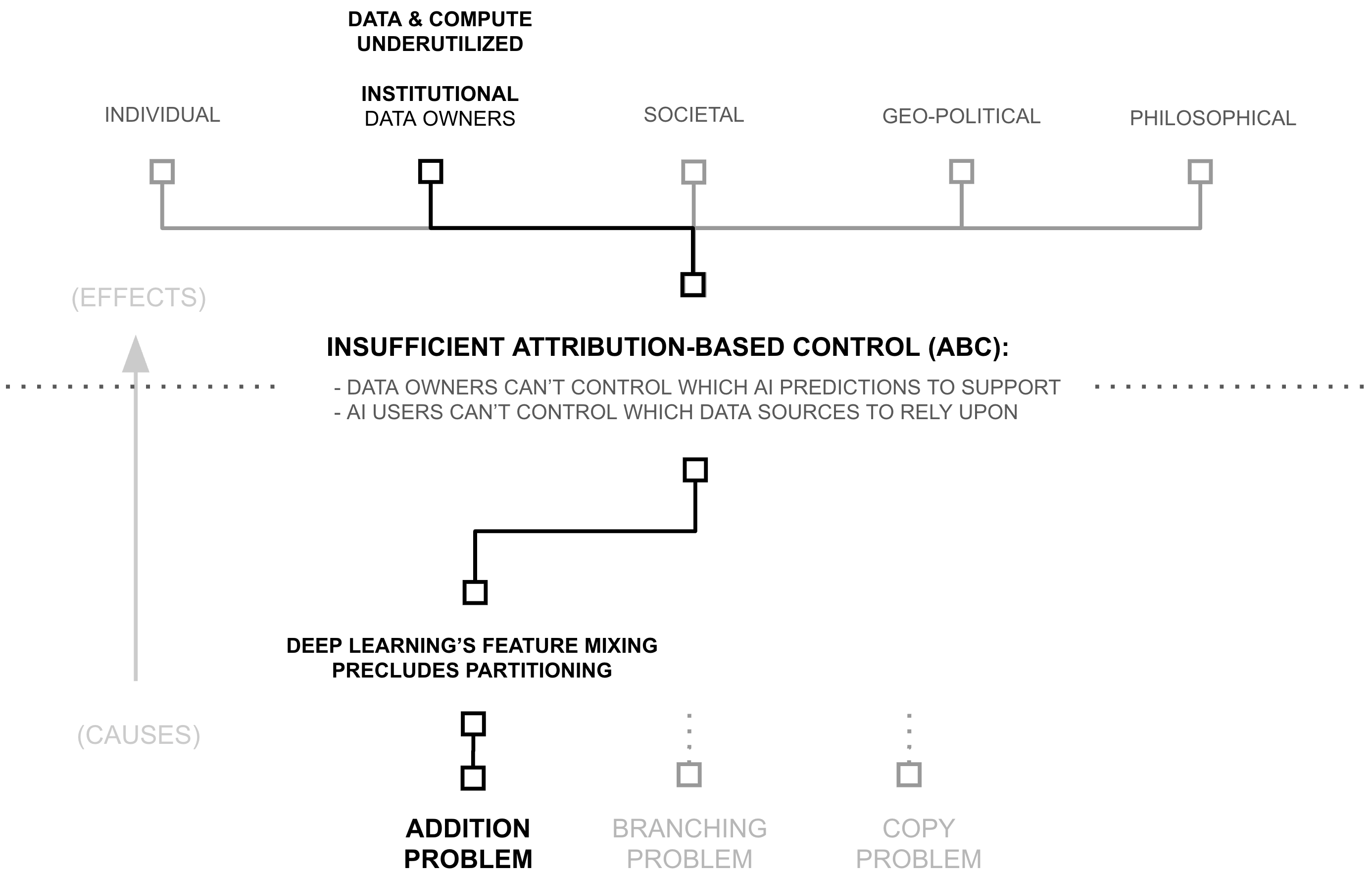
The Search for Root Causes (Three "Whys")
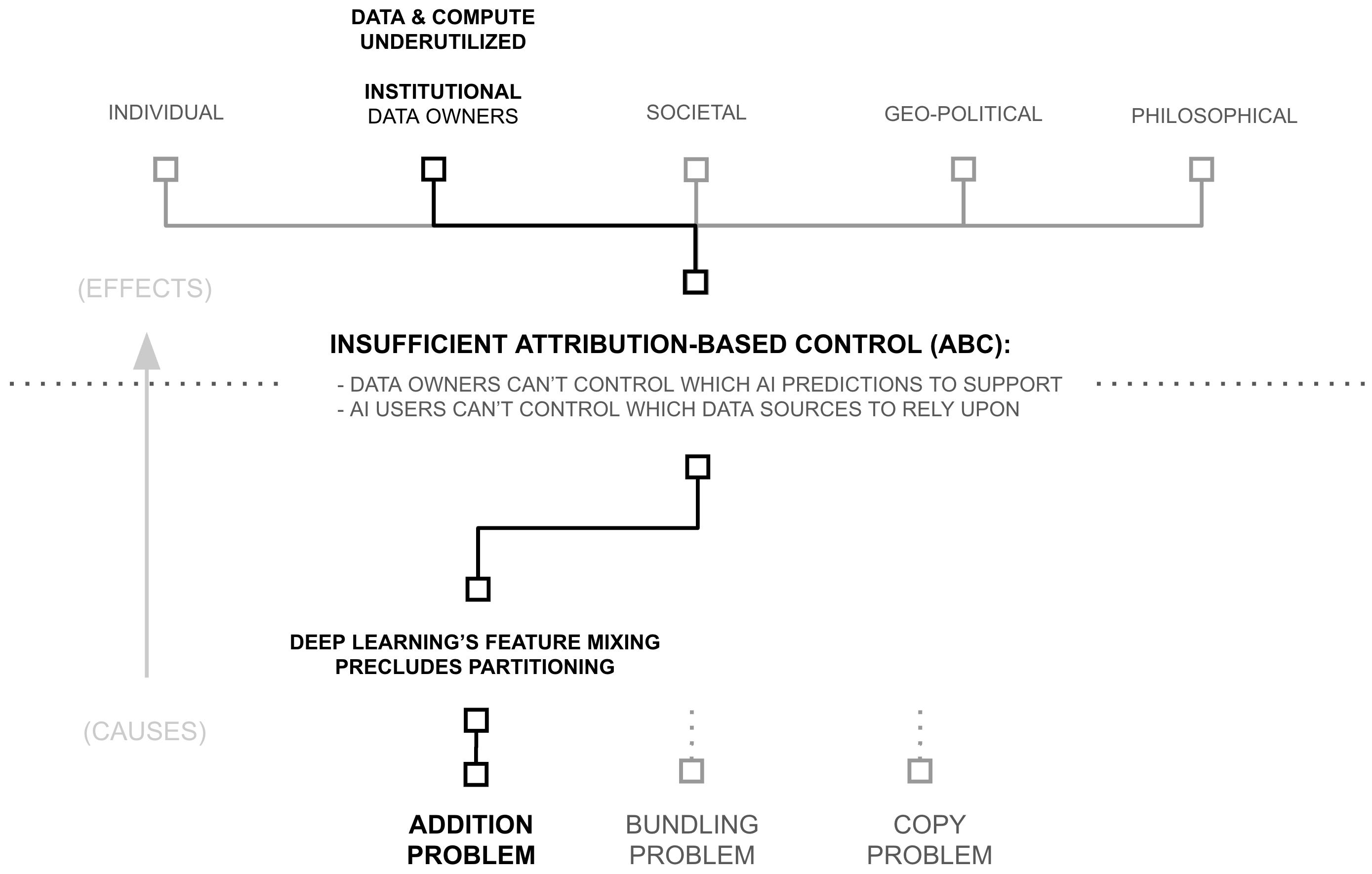
The previous section revealed a paradox: despite widespread beliefs of data and compute scarcity, AI systems access less than one millionth of digital resources, and an untold microfraction of the world’s information broadly. This under-utilization raises a critical question: if more data and compute directly improves AI capabilities through scaling laws, why do AI systems use such a tiny fraction of what’s available? The answer lies in a cascade of technical and institutional barriers, each revealing a deeper ”why” that must be understood:
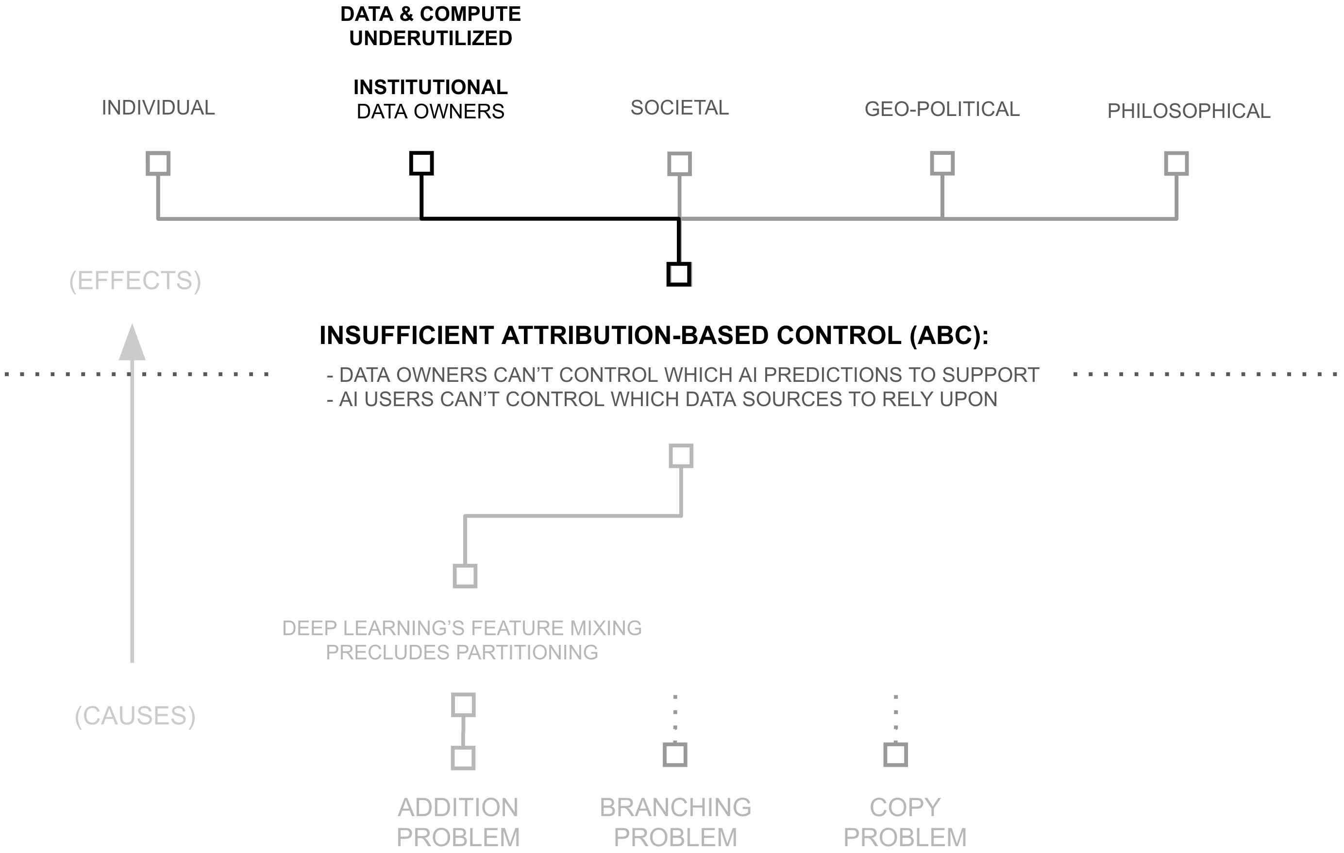
- First Why: Attribution-based Control
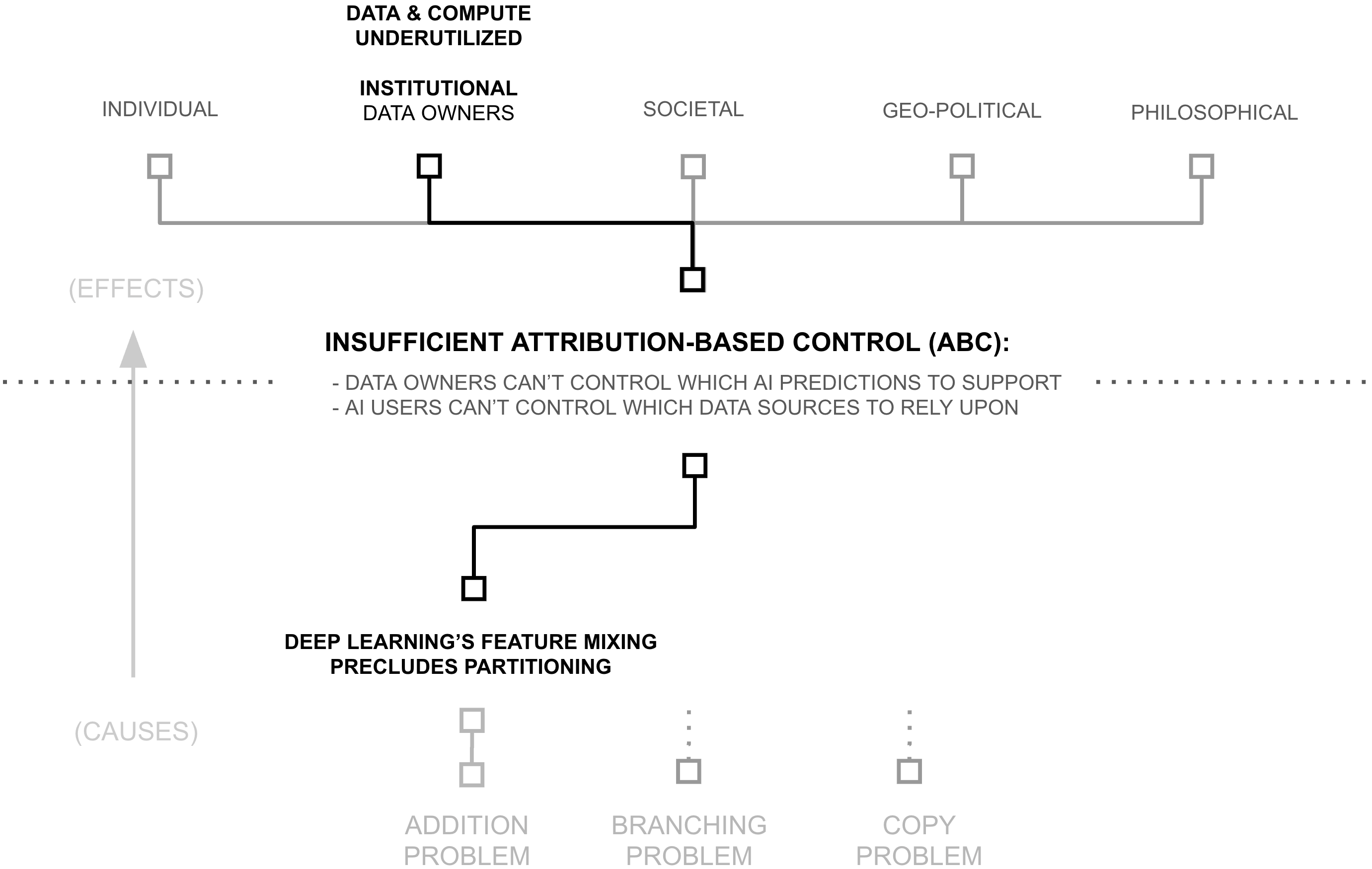
- Second Why: Deep Learning's Feature Mixing Precludes Partitioning
- Third Why (Root Cause): Addition of Source-Separable Concepts
As we follow this chain of questions, we’ll see how each answer reveals a deeper technical challenge. More importantly, we’ll discover how recent breakthroughs in cryptography, deep learning, and distributed systems have already created solutions to these challenges (solutions which remain largely unrecognized by the AI community).
First Why: Attribution-based Control
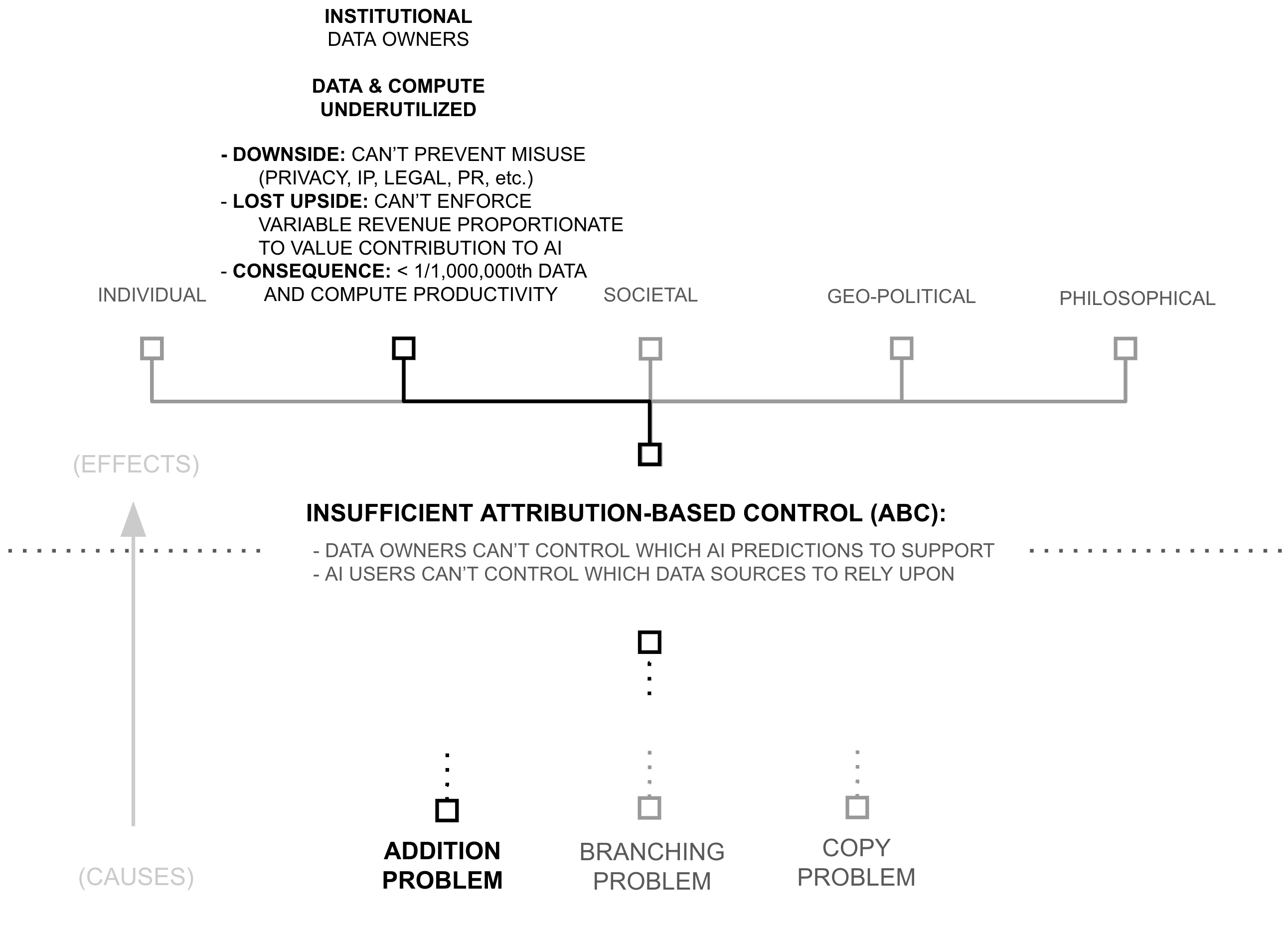
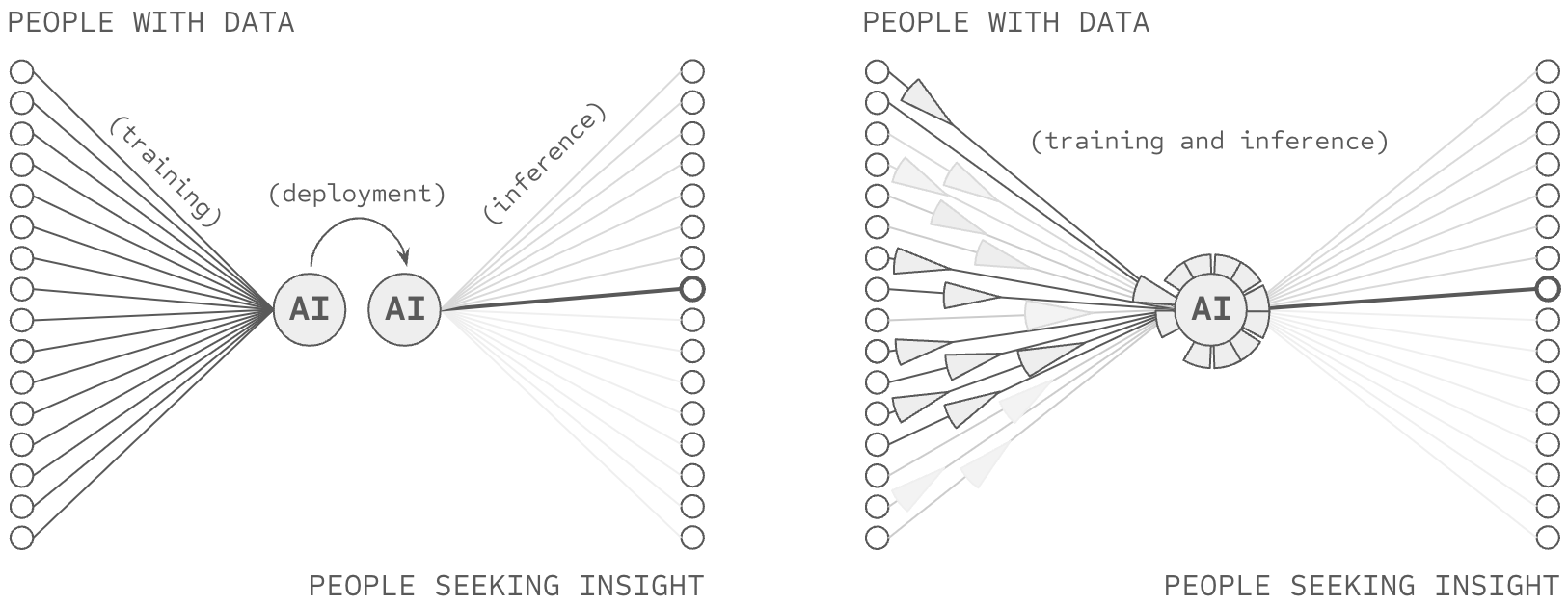
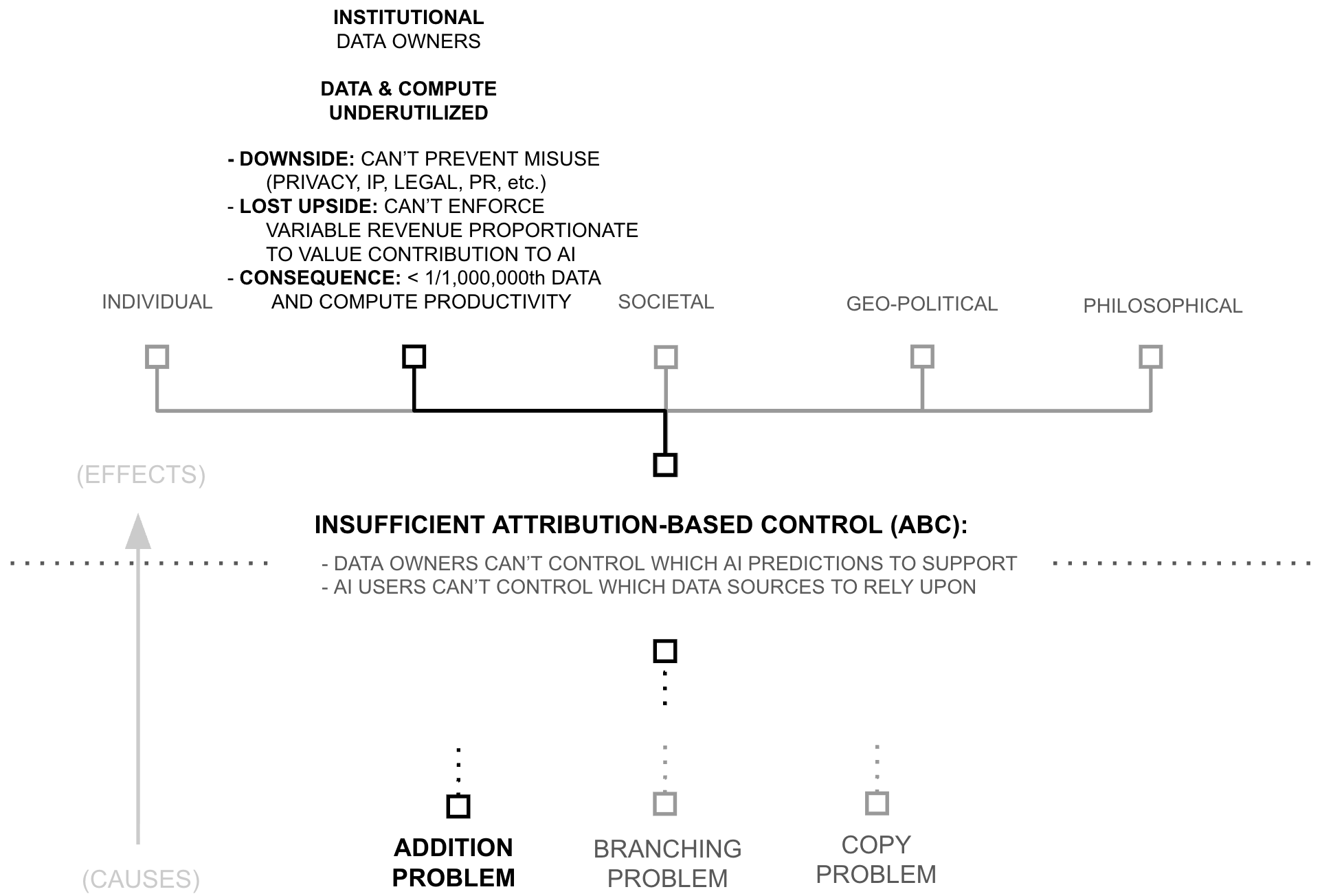
The previous section revealed significant inefficiencies in the training of AI systems: 6+ orders of magnitude in underutilized data and compute. While there may be multiple contributing factors to these constraints, this thesis and chapter examines one particular root cause: AI’s inability to provide attribution-based control (ABC). An AI model possesses attribution-based control when two properties are true: data sources control which AI predictions they support, AI users control which data sources they rely upon for an AI prediction. Following this definition (Definition 1.1.1), ABC implies certain architectural properties as novel requirements:
- Source-Partitionable Representations: Knowledge within an AI system is
partition-able
by source, otherwise sources lose control when their information is mixed, requiring:
- Source-Partitionable Inference: Partitions are independently usable at inference, otherwise users can’t select specific sources and sources can’t participate irrespective of the decisions of other sources
- Source-Partitionable Training: Partitions are independently trainable, otherwise sources can’t update their contributions without requiring other sources to do so.
- Rapid Partition Synthesis: Partitions are rapidly synthesize-able during inference, otherwise collective insights which are only learnable via information from multiple sources cannot be realized in production AI systems.
Frontier AI systems lack these properties. Yet, if these properties were achieved, attribution would be achieved and aforementioned problems regarding data and compute productivity would be impacted. Let’s examine each in detail, linking each problem to attribution-based control.
ABC and Compute Productivity (6+ OOM)
ABC would address compute productivity issues along two dimensions: access and learning structure. Regarding structure, successful ABC would necessarily provide a means to structure the learning and representation process, reducing re-training, forward propagation, redundancy, and catastrophic forgetting. Regarding access, ABC would provide a means to overcome incentive issues presently siloing the world’s compute resources. Let us consider these claims in the context of inference and learning.
2-3 OOM: Inefficient AI inference
A Library Analogy
Consider a library wherein a librarian reads every book in the library whenever they need to answer a question, including reading multiple copies of the same book and pretending to read an empty book whenever shelves contain empty sections.
A solution to attribution-based control would necessarily reconfigure the library to fetch information based on its source (book or author). While such a solution might be challenging, if it successfully delivered capable predictions, it would necessarily do so while skipping an enormous amount of wasted computation. This is because ABC is not actually about selecting the sources one desires (normal full forward propagation already does this), its actually about ignoring all the books you don’t want. ABC requires making an AI inference while skipping an enormous amount of wasted computation, because (to return to the analogy) it would involve training the librarian on how to skip reading the entire library when making a prediction... and only fetch information from specific, relevant sources (i.e. books).
Thus, while ABC’s definition might not appear to require an increase in computational efficiency, its definition directly requires that a vast amount of information not be included in the computational process, reducing the need to compute over that information.
Recall that current AI models must activate vast numbers of parameters for every prediction because they struggle to pre-identify which parameters are storing relevant information to the present query; they struggle with sparse forward propagation. While various approaches to sparse AI exist, successful ABC would necessarily enable one particularly compelling form of sparsity: source-based sparsity (i.e. source-based partitioning). Consequently, if an AI model could forward predict based on a relevant subset (i.e., the top 10) of many (i.e. billions) of sources, then it is very likely to also greatly reduce the computational complexity involved in forward propagating, because it would be forward propagating through vastly less information.
RETRO and ATLAS demonstrate the minimum scale of such a breakthrough. By maintaining source-based partitions through their database architecture, they achieve equal performance while activating only 2-4% of the parameters of similarly performant dense models (Borgeaud et al., 2022; Izacard et al., 2023).
Similarly, recall how current models process some combination of redundant copies of knowledge and empty regions of parameter space during inference. While there are many approaches to reducing these forms of waste (e.g., distillation, compression, etc.), successful ABC would necessarily enable one particularly compelling way to avoid copies or empty space: source-based partitioning. If an AI model could forward predict based on a relevant subset (i.e., the top 10) of many (i.e., billions) of sources, then tuning the number of sources being relied upon could also tune the redundancy being used in forward propagation. Meanwhile, ensuring that the partitions being leveraged for forward propagation were relevant to the query would combat the risk of forward propagating empty space 2.
RETRO and ATLAS demonstrate these principles through their database architecture, showing how source-based organization can naturally eliminate redundant processing and avoid computation on irrelevant parameters while maintaining model capability. They also demonstrate the ability for such partitioning to increase the number of samples being used against a dense (i.e. non-partitioned) section of the network, reducing empty space. Yet as significant as these inference inefficiencies are, they pale in comparison to the waste in how AI systems learn.
6+ OOM: Underutilized and Inefficient Compute in AI Learning
Recall that current AI models must retrain entirely from scratch when updating their knowledge, because of problems such as catastrophic forgetting (Kemker et al., 2018). While various approaches to incremental training exist, successful ABC would necessitate one particular solution: source-partitioned retraining. Consequently, if an AI model can train source-separated subsections of its weights, it can re-train them as well, and it is very likely to also greatly reduce the computational complexity involved in the re-training process, because it would be re-training vastly fewer parameters at a time. RETRO/ATLAS demonstrate one such approach, wherein re-training can be done with the computational complexity involved in adding or removing vector-embeddings from a database.
Similarly, recall how current training processes waste compute in multiple ways: through redundant copies of the same knowledge, through activation of irrelevant parameters, and through inefficient parameter density. While various approaches to training efficiency exist, successful ABC would necessarily enable compelling means to overcome these problems (as already described in the previous section describing ABC’s impacts on inference).
Additionally, these ABC opportunities further compound when we consider how compute is distributed across organizations. Consider our library analogy once more: libraries don’t each maintain copies of every book ever written; they form networks to share resources efficiently. In contrast, frontier AI models are created by a host of organizations around the world, each re-paying the cost of creating an AI model (most of which are trained on largely the same data).
Successful ABC may activate an economic incentive addressing this waste 3 . At the present moment, frontier AI models are economic bundles, marketed under a story which itself is an economic bundle: artificial general intelligence. Because of this, if one AI company re-trains the capabilities of another company (e.g. spending $200M on compute) and then adds a bit more to it (e.g., another $10M in data and compute), an end user must then choose between that full economic bundle and another full economic bundle. This creates a situation wherein companies effectively have to pay the minimum amount to catch up to the leading position and then extend some beyond it.
2 Additionally, if successful ABC reduced the number of parameters being used as a result of these other techniques, then it would also increase the number of samples being applied to each set of dense parameters — perhaps reducing the opportunity for empty vector space (more on this later)
3 This hypothesis has been somewhat validated by OpenMined in early pilots of ABC-enabled AI systems with publishers, but this research is as-of-yet unfinished
A Library Analogy
Consider a new library which doesn’t yet have any books. To load the library in the style of AI, a librarian would first build tens-of-thousands of libraries and print copies of books into each one (i.e. signifying both the redundant training of models by many companies and the hyperparameter sweeps occurring within each one). Then, within each library, a librarian would first load all the shelves (of which there are a fixed number) books containing random strings of letters (i.e., initialize a model randomly). Then, the librarian would select the first book to load into the library, pretend to read every word in every one of the random books, and after that was done, select which book to replace with the book being loaded into the library, casting the book being replaced onto the floor. The process would repeat until all of the books had been loaded... with a catch. Each time the book being thrown on the floor wasn’t a random book (but was a real book) that real book then needs to go through the process again itself. And in the end, if the library wasn’t big enough to contain all the books, all the libraries would be destroyed, all the copies of books burned, and everyone would re-build bigger libraries to hold the vast and growing collection of books.
A solution to attribution-based control would necessarily reconfigure the library to load information based on its source (book or author). While such a solution might be challenging, if it successfully delivered capable predictions, it would necessarily do so while skipping an enormous amount of wasted computation. Instead of each library creating a collection big enough to hold the world, the vast collection of the world’s books could be divided among the libraries (perhaps with some mild redundancy). Each library could then organize their books by the dewey decimal system, measuring how big each section in their library needs to be in order to hold the sections they are meant to store. After these measurements were completed, the building could be constructed, the books loaded in their proper places, and the job could be completed.
And in this way, the librarian could avoid storing all the world’s information in their own library, re-building libraries from scratch, reading all the books in the library over and over, loading in many copies of the same book, loading in empty or random books, and re-loading books which no longer fit on the shelves they’re loading. Taken together, while ABC’s definition might not appear to require an increase in computational efficiency, its definition directly requires that a vast amount of information not be processed during iterative steps in the training process, reducing the need to compute over that information. In some cases, ABC implies the elimination of iterative processes altogether.
However, successful ABC would modularize the initial capability, such that some percentage of the original $200M could be inherited from previous models and then extended with new capabilities. Given the immense costs involved, such a modularization breakthrough would constitute an enormous economic pressure. If firms pedantically chose to re-pay the cost to train their own from scratch, recreating 90% of the modules which already exist in the market, they would incur very high costs which must correspond with very high prices to recoup those costs. Inversely, a startup which came along and inherited the 90% produced by others, paying only for their specialization, would (all else equal) be able to charge lower prices, and win in the market.
From a compute efficiency standpoint, the prospect of cross-market weight-reuse translates directly into the sharing of compute costs for training AI systems. Industry analysis reveals the potential impact: no single AI provider controls more than 5.57% of global compute capacity. Thus, since source-based partitioning could unlock this siloed compute by enabling controlled sharing of specialized knowledge, it could increase effective compute by 17.95x (100/5.57) or more because organizations would waste fewer resources re-computing features which are already commoditized in the market. Taken together, economic unbundling would plausibly drive specialization and more efficient use of compute resources in the market.
While various approaches to these inefficiencies exist, solving ABC would necessarily enable one comprehensive solution path. Note that this is not saying that ABC is the solution, merely that ABC is difficult because it would involve solving these other difficult challenges... because ABC requires that sources maintain control over their contributions while enabling rapid synthesis. Taken together, any solution to ABC solution must provide:
- Selective retraining instead of full rebuilding (68x+ improvement)
- Efficient computation during training (25-50x+ improvement)
- Reduced parameter redundancy through source-based organization (5-10x+ improvement)
- Specialization with controlled sharing (17.95x+ improvement)
- Organization averting catastrophic forgetting (17.95x+ improvement)
Industry analysis and empirical results suggest the combined impact could be dramatic. When these improvements compound multiplicatively, they point to potential training efficiency gains of 6+ orders of magnitude. Yet these numbers, as striking as they are, point to something more fundamental: our failure to maintain attribution in AI systems coincides with a broader acceptance of wasteful practices as inevitable. More than a technical issue, the inefficiency of AI training is a symptom of how we’ve structured AI computation. While other solutions may exist, attribution-based control offers one path to reimagining how AI systems learn and compute, potentially unlocking orders of magnitude more efficiency in the process.
How Failing ABC Siloes Data (6 OOM)
Recall that current AI models can only train on data they can access, which is dominated by data available to the public over the internet. Consequently, AI models almost certainly train on less than 1/1,000,000th of the digitized information in the world because they cannot access the other 99.9999%, which remains hidden amongst the world’s 360 million companies, 8+ billion citizens, etc. (Bogwasi 2025).
While various approaches to data access exist, successful ABC would necessarily enable one compelling solution: controlled data sharing. We take as an assumption that the world’s data owners have some uses in the world they would support (for which their data could be useful). We take as a second assumption that a significant portion of those sources are hidden because the incentives are not sufficient for them to support — or more crucially because the negative consequences would be too great, that their data might not just activate the uses they wish to support, but that it would also activate mis-uses (concerns regarding privacy, security, IP, competition, legal risks, etc.).
Successful ABC would necessarily enable one particularly compelling form of data sharing. The ability for a data source to decide which AI predictions to support is (almost tautologically) the ability for a data source to enable uses while averting mis-uses. Consequently, AI empowered by ABC may activate vastly more data than is presently available. One could argue that truly successful ABC would constitute an incentive shift attracting all of the world’s data to be pulled into at least some AI predictions.
The potential impact is staggering. While frontier AI models train on carefully curated web scrapes on the order of 180 TBs (and the public web plausibly less than common crawl’s largest copy, 450 TBs) the world’s total digital data is estimated to reach 180 zettabytes by 2025. This six-to-nine orders of magnitude difference represents all the data locked behind organizational boundaries, including some data of immense value (e.g. financial data, health data, environmental data, etc.).
RETRO and ATLAS demonstrate part of potential path forward, demonstrating a type of partial ABC at scale by training AI models which query from a database. Certain extensions (such as those suggested in this thesis) could take this further to enable full attribution-based control, and the shifting of incentives around data sharing.
Synthesis: Attribution as a Path Forward
The previous sections revealed two significant inefficiencies in current AI systems: 6+ orders of magnitude waste in compute and 6+ orders of magnitude in untapped data. While there may be many approaches to addressing these inefficiencies, this thesis focuses on attribution-based control as one solution path. As we’ve seen, solving ABC (if such a solution exists) would necessarily enable both efficient compute through source-based partitioning and broad data access through attribution preservation.
Yet this raises a deeper question: if ABC offers such compelling benefits, why don’t current AI systems maintain attribution? The answer, as we’ll see in the next section, lies in how neural networks fundamentally process information. The unconstrained mixing of features during training makes it impossible to partition knowledge by source, revealing our second ”why”: deep learning’s feature mixing precludes the very partitioning that ABC requires.
Second Why: Deep Learning's Feature Mixing Precludes Partitioning
The previous section revealed how solving attribution-based control would necessarily enable massive data and compute gains in AI systems. Yet this raises a deeper question: why do current AI systems fail to maintain attribution in the first place? The answer lies in deep learning’s foundational premise: algorithms should learn everything from scratch through layers of (largely) unrestricted feature mixing on raw data (Goodfellow et al., 2016).
This commitment to unrestricted learning manifests in how neural networks fundamentally process information. Through operations that combine and mix information at every step (from layer computations to weight updates to knowledge accumulation) neural networks create increasingly complex representations of patterns in their training data. While this flexibility enables powerful pattern recognition, it creates a fundamental problem: features become stored in a disorganized, obfuscated way within the deep learning model... a black box.
Consider what happens when a neural network learns to recognize cats. Rather than storing clear, interpretable features like ”pointy ears” or ”whiskers”, the network distributes this knowledge across its weights in complex, entangled patterns (Le 2013). This unrestricted mixing of features makes post-hoc source-based partitioning impossible (at the present moment):
- Features can’t be attributed to specific sources (preventing data control)
- Knowledge can’t be updated independently (requiring full retraining)
- Computation can’t be selectively activated (forcing dense inference)
- Resources can’t be efficiently shared (blocking specialization)
The research community has made extensive efforts to address these limitations. Recent work has attempted to trace predictions back to training data through influence functions, remove specific datapoints’ influence through machine unlearning, and develop various attribution methods to reverse engineer the source-prediction relationship (Nguyen et al., 2024). Yet despite these attempts, both influence functions and unlearning remain unsolved challenges in the literature. So far, the relationship between sources and predictions has been irreversibly compressed during training, and no amount of post-training intervention has successfully restored these lost connections.
The consequences are severe. New models like GPT-5 cannot inherit features from predecessors like GPT-4... they must relearn basic patterns from scratch. Even during inference, models must activate vast parameter spaces for every prediction, unable to pre-identify which features are relevant (and only forward propagate those features). These inefficiencies aren’t mere implementation details that clever algorithms might solve. They stem from something more fundamental about how deep learning processes information.
Yet this raises an even deeper question: why does feature mixing obfuscate attribution-based control? The answer, as we’ll see in the next section, traces back to deep learning’s most basic mathematical operation and how it fundamentally precludes the partitioning that ABC requires.
A Library Analogy
Consider a library wherein all of the books have had their covers removed, their table of contents erased, and their chapters torn out and shuffled amongst all the books. Consequently, when someone wants to answer a specific question, they have to read through the entire library searching for relevant information for their query.
Deep learning stores information in a similar way, with so-called distributed representations spreading concepts across many neurons... each of which is unlabeled (i.e. ”hidden”). Far from an accident, this form of learning is at the center of deep learning’s core philosophy, the unrestricted learning of dense, hidden features.
Third Why (Root Cause): Addition of Source-Separable Concepts
The previous section revealed how deep learning’s feature mixing precludes the partitioning required for attribution-based control. Yet this raises our final ”why”: what makes this mixing fundamentally irreversible? The answer lies in deep learning’s most basic mathematical operation: addition.
Addition might seem like an implementation detail, but it fundamentally prevents recovering source information. When values combine through addition, the result does not uniquely determine its inputs—multiple distinct source combinations produce identical outputs:
Non-Injectivity of Addition
Addition is not injective: for any sum y, there exist infinitely many distinct pairs (x1, x2) and (x'1, x'2) such that x1 + x2 = y = x'1 + x'2 where (x1, x2) ≠ (x'1, x'2).
This non-injectivity means that observing the sum provides no information about which specific sources contributed. Consider the contrast with concatenation:
Concatenation vs Addition
Concatenation preserves sources:
"1" ⊕ "6" = "16"
"2" ⊕ "5" = "25"
(distinct inputs → distinct outputs)
Addition erases them:
1 + 6 = 7
2 + 5 = 7
(distinct inputs → identical outputs)
When partitions are known, concatenation of numbers is injective; different inputs produce different outputs, allowing source recovery. Addition is not; the output 7 could arise from 1 + 6, 2 + 5, 3 + 4, 0 + 7, or infinitely many other combinations. This non-injectivity is the mechanism through which deep neural networks erase attribution information: once gradients from different sources are summed into shared parameters, no function of those parameters can recover which sources contributed what information.
And neural networks use addition extensively: combining features between layers, aggregating gradients during backpropagation, and updating weights during training. Each addition irreversibly combines information, destroying the provenance of where that information came from and how it was interpreted.
A natural solution might seem possible: why not just track every operation during training ... while also doing these additions? Unfortunately, this approach fails for three fundamental reasons:
First, in models like GPT-3, through forward and backward propagation, each example’s information eventually touches every weight in the network. Even tiny weight changes alter how future examples flow through the network, creating cascading effects that can amplify initially small influences (related: vanishing and exploding gradients (Hochreiter 1998; Hanin 2018)).
Second, these influences compound exponentially and recursively, creating higher order all-to-all relationships between inputs and weights as they do. Consider the mathematics of weight updates for a weight update function g, weights and data at time t as w t and x t :
w t+1 = g(wt, xt)
w t+2 = g(g(wt, xt), xt+1)
w t+3 = g(g(g(wt, xt), xt+1), xt+2)
The number of potential attribution paths grows as Ω(w · n)t , where w is the number of weights, n is the number of examples, and t is the number of steps.
Third, this exponential growth makes exact attribution computationally intractable. The most capable language models frequently leverage just under 1% of their parent organization’s AI training budget (see Appendix I and II for details). Thus, tracking the full web of dependencies (every interaction, every update, every influence path) would require many orders of magnitude more compute than is available to the largest tech firms.
These three barriers (information loss through addition, exponential propagation of influences, and computational intractability) combine to create a fundamental limitation. No amount of clever engineering can fully recover what addition has destroyed. This mathematical reality explains why attempts at machine unlearning and influence functions remain fundamentally limited: they try to reconstruct what addition has already erased.
The Root Problem: The implications are significant. Without the ability to track sources through training, we cannot provide the attribution that ABC requires. Without attribution, we cannot enable the partitioned sharing and use of data and compute that could unlock orders of magnitude more AI resources. Addition itself blocks the very data and compute gains described earlier in this chapter, and holds up the many problems described in Chapter 1.
A Library Analogy
Consider a library wherein all of the books have had their covers removed, their table of contents erased, and individual sentences on each page torn out into their own strips. Now imagine that each word in each strip is converted into a number ”aardvark = 1”, ”abernathe = 2”, and so forth. And then imagine that each of these strips from the whole library is shuffled around, and groups of strips are placed back in the coverless books. Yet, instead of each strip being glued in place, it is first combined with many other strips, adding their respective numbers together. Consequently, when someone wants to answer a specific question, they have to read through the entire library searching for relevant information for their query, first by converting their query into numbers and then attempting to match it to numbers found in the books.
Deep learning stores information in a similar way, with so-called distributed representations spreading concepts across many neurons... each of which is unlabeled (i.e. ”hidden”). Far from an accident, this form of learning is at the center of deep learning’s core philosophy, the unrestricted learning of dense, hidden features which are formed through many successive additions.
Third Hypothesis (Root Solution): Concatenating Along Natural Boundaries in Data Sources Enables Attribution
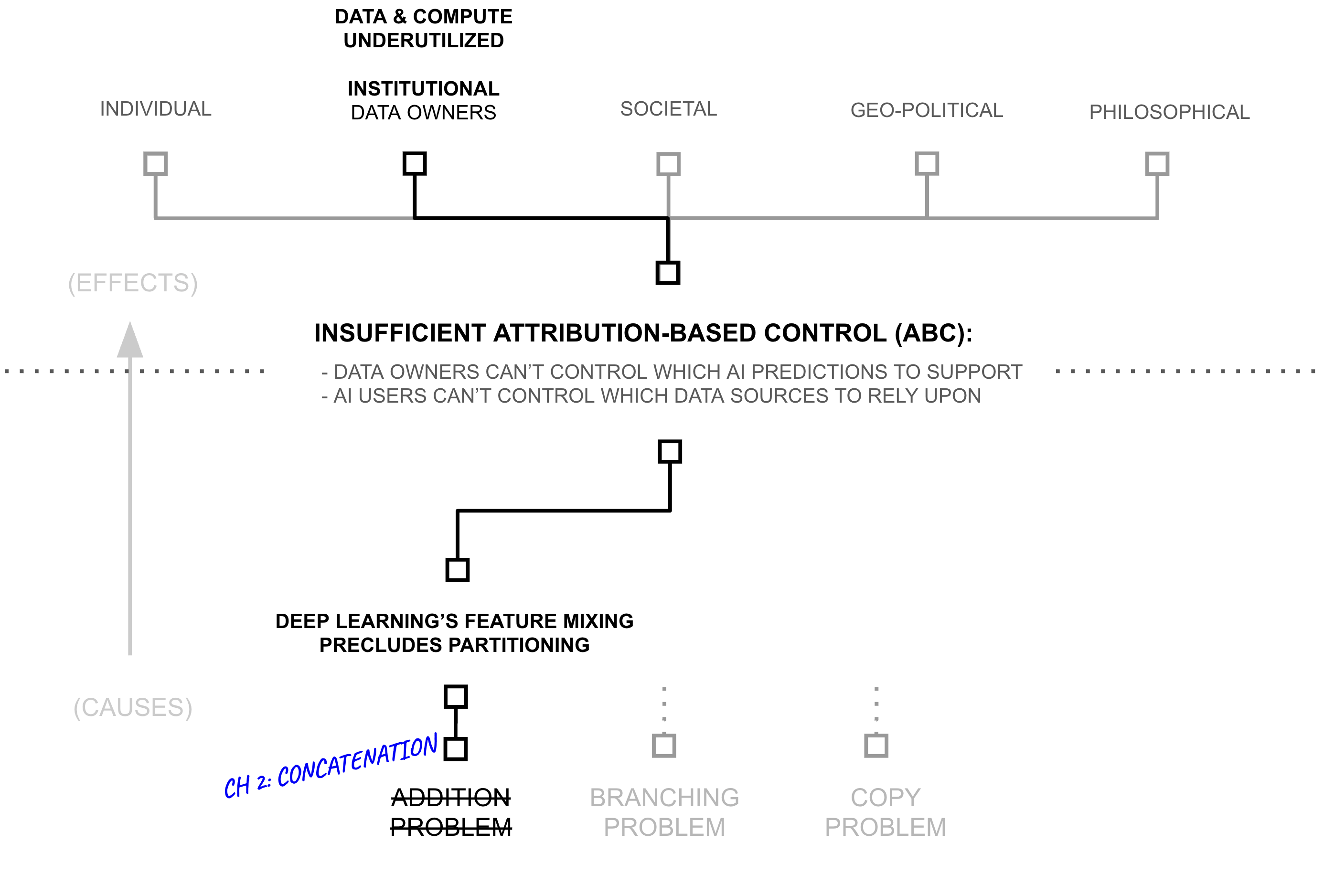
We now continue by constructing a hypothesis (the “Third Hypothesis”) which corresponds to the Third Why, which will support the Second Hypothesis addressing the Second Why and so forth. The previous sections revealed how addition in deep learning creates a fundamental barrier to attribution. Yet examining why addition fails suggests a testable hypothesis: can we significantly reduce the use of addition, perhaps swapping it with concatenation?
Deep learning’s central hypothesis would suggest we can’t, that features need to densely mix (using addition) in order to learn the powerful correlations and representations that give deep learning its predictive capability. However, presumably deep learning maps multiple distinct concepts into a shared feature when those two concepts are related (Krizhevsky et al., 2012). For example, a deep learning model which classifies images might have features which detect ears, fur, and eyes — features which would be useful for modeling many different animals which possess these related concepts (Zeiler and Fergus 2014). However, as these features are not laid out in advance, deep learning needs to densely mix its features in order to discover these related patterns across training datapoints. That is to say, perhaps over-zealous dense feature mixing is more about training than inference
Yet, perhaps deep learning is over-zealous in its feature mixing, opening itself to representation power which could mix any feature with any other when in the real-world not all concepts are closely related. That is to say, not all concepts require that level of general representation power. Perhaps some concepts are actually unrelated to one another, such that some proportion of dense feature mixing in deep learning is superfluous
That said, some concepts are densely mixed, while others are clearly less so. Some information patterns appear ubiquitously: basic rules of grammar that structure language, logical operations that appear in reasoning, morphological patterns which make up words, edges and corners in images, etc. Elements like these are frequently reused across almost every data point, appearing in many billions of documents, images, audio, and videos. Such dense patterns suggest unrestricted mixing through addition may be appropriate for a core subset of features. Their ubiquity also makes attribution less critical; they represent shared computational tools rather than source-specific claims about the world. While perhaps not formally stated, noted researcher Andrej Karpathy recently suggested a similar concept when referring to a future LLM “cognitive core”:
The race for LLM “cognitive core”—a few billion param model that maximally sacrifices encyclopedic knowledge for capability. It lives always-on and by default on every computer as the kernel of LLM personal computing. Its features are slowly crystalizing:
- Natively multimodal text/vision/audio at both input and output.
- Matryoshka-style architecture allowing a dial of capability up and down at test time.
- Reasoning, also with a dial. (system 2)
- Aggressively tool-using.
- On-device finetuning LoRA slots for test-time training, personalization and customization.
- Delegates and double checks just the right parts with the oracles in the cloud if internet is available
It doesn’t know that William the Conqueror’s reign ended in September 9 1087, but it vaguely recognizes the name and can look up the date. It can’t recite the SHA-256 of empty string as e3b0c442..., but it can calculate it quickly should you really want it.
What LLM personal computing lacks in broad world knowledge and top tier problemsolving capability it will make up in super low interaction latency (especially as multimodal matures), direct / private access to data and state, offline continuity, sovereignty (“not your weights not your brain”). i.e. many of the same reasons we like, use and buy personal computers instead of having thin clients access a cloud via remote desktop or so.
— Andrej Karpathy[link]
In contrast, perhaps most information is encyclopedic and appears sparsely: specific facts about the world, domain expertise in particular fields, claims made by individual sources, etc. The capital of France, the rules of chess, statistics about pizza... each appears in distinct contexts with limited overlap. As Chomsky noted in linguistics (Chomsky 2014), while we use common patterns to express all knowledge, the knowledge itself often remains naturally partitioned by topic, and when documents are topic specific... by source.
Let us assume for a moment that this is true. If so, then in theory some section of a neural network could be made sparse, namely the part of the neural network which stores concepts which are largely decoupled from the rest of a neural network’s knowledge (facts, domain expertise, semantic information, etc.). Perhaps this section could use less addition (and more concatenation), enabling sparsity which could drive attribution. Meanwhile, another part of the neural network might need to remain dense, storing and synthesizing concepts which are ubiquitous across a statistical distribution (logic, reasoning, syntax, etc.).
The key question: how would one go about training a neural network which successfully partitioned information into sparse and dense sections?
A key insight of this chapter is that techniques from privacy-preserving machine learning, particularly differential privacy (DP) (Dwork et al., 2006), provide a principled way to measure and control which features benefit from dense mixing versus sparse representation. Differential privacy quantifies how much a model’s outputs depend on any individual training example:
(ε, δ)-Differential Privacy
A randomized mechanism $\mathcal{M}: \mathcal{D} \to \mathcal{R}$ satisfies (ε, δ)-differential privacy if for all adjacent datasets $D, D' \in \mathcal{D}$ (differing in one example) and all subsets of outputs $S \subseteq \mathcal{R}$:
$\Pr[\mathcal{M}(D) \in S] \leq e^\epsilon \cdot \Pr[\mathcal{M}(D') \in S] + \delta$
where small ε indicates strong privacy—outputs barely depend on any individual example.
The parameter ε provides a quantitative measure of individual example influence on outputs. This same measure can serve three distinct control objectives:
Three Regimes of Influence Control
For a mechanism M, examples e, and thresholds 0 < τmin < τmax:
- Privacy (constrain influence): Enforce εe < τmin for all examples, guaranteeing that individual examples cannot be distinguished through their influence on outputs
- Measurement (track influence): Compute εe for each example, enabling quantification of which examples influence which outputs, without enforcing bounds
- Attribution (ensure influence): Enforce εe > τmax for specified examples, guaranteeing that certain examples have measurable influence on outputs
These three regimes serve different stakeholder needs. Data owners might seek differential privacy (ensuring their data cannot be identified in model outputs), differential measurement (understanding their data’s contribution), or differential attribution (guaranteeing their data influences predictions). Users might seek privacy (preventing their queries from revealing information) or attribution (ensuring they can identify which sources influenced their results). The same mathematical framework (DP’s ϵ parameter) enables each form of control.
Given differential privacy’s use in deep learning (e.g., (Abadi et al., 2016)), this framework suggests an architectural insight: a neural network serving diverse stakeholders requires the capability to enforce different ϵ regimes for different information. Information requiring privacy (small ϵ) can pass through privacy-constrained layers with dense mixing via addition. Information requiring attribution (large ϵ) must route through pathways preserving source identity via sparse concatenation. Information requiring measurement sits between these extremes, with ϵ tracked but not bounded. The model’s optimization pressure, when constrained to respect these different ϵ regimes, might naturally partition information accordingly. This framework suggests two testable predictions:
First, features with high source-specific attribution should cluster naturally by source, while features with low attribution should appear consistently across sources. Recent work with RETRO and ATLAS provides initial evidence for this prediction, showing how knowledge naturally separates into general computational patterns (the Transformer reading from a database of vectors, similar to Karpathy’s “cognitive core”) and source-specific information (the database of vectors).
Second, respecting these natural boundaries through architectural choices might enable more efficient computation. If most information is sparsely distributed, then forcing it through dense addition operations wastes significant compute. Models that preserve sparse patterns through concatenation while sharing dense patterns through addition should achieve better computational efficiency. Again RETRO and ATLAS provide early evidence of this ability, wherein information within their vector database is concatenated (i.e. in different rows of the database), while information in the neural network consuming from the database is densely stored within Transformer weights.
The next section builds on this hypothesis, suggesting how these natural boundaries in information usage could enable new approaches to AI development. If correct, this could resolve the tension between deep learning’s powerful pattern recognition and the need for attribution-based control in AI systems.
A Library Analogy
Consider a library wherein all of the books have had their covers removed, their table of contents erased, and individual sentences on each page torn out into their own strips. Now imagine that each word in each strip is converted into a number ”aardvark = 1”, ”abernathe = 2”, and so forth. And then imagine that each of these strips from the whole library is shuffled around, and groups of strips are placed back in the coverless books. Yet, instead of each strip being glued in place, it is first combined with many other strips, adding their respective numbers together. Consequently, when someone wants to answer a specific question, they have to read through the entire library searching for relevant information for their query, first by converting their query into numbers and then attempting to match it to numbers found in the books.
Following the analogy, differential attribution ensures that each strip of numbers remains separated (instead of added) into each other strip, and preserved within the same book as before, partitioning data in a way which might be indexed by source or topic.
Second Hypothesis: From Deep Learning to Deep Voting with AI Recycling and Src-specific Intelligence Budgets
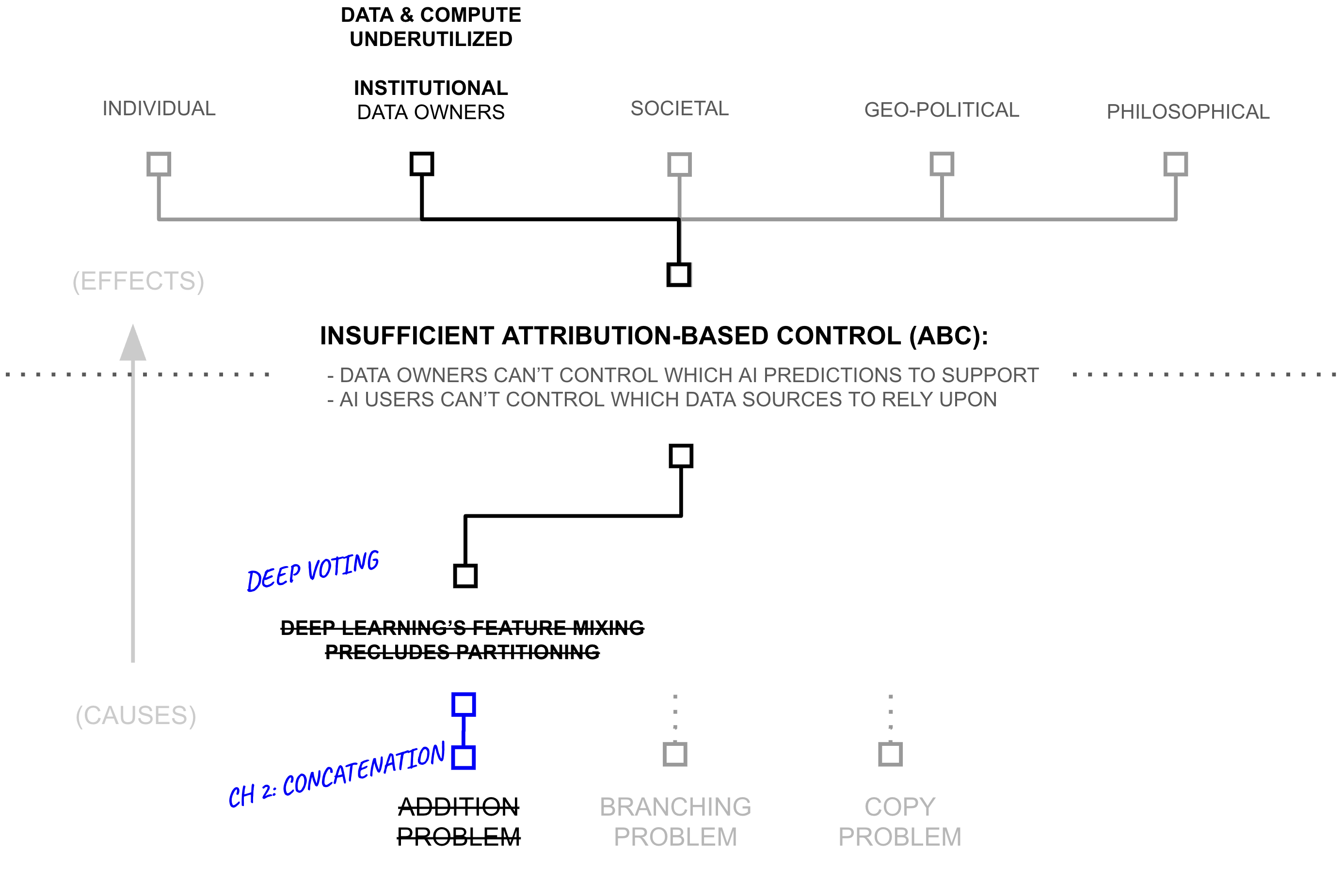
The previous section revealed how privacy mechanisms might naturally separate dense from sparse information patterns. Yet this theoretical insight raises a practical question: how do we actually implement the measurement and control regimes we defined? The definitions in the previous section assumed worst-case bounds (requiring that ϵ constraints hold for all pairs of neighboring datasets). But attribution-based control requires the opposite: not uniform bounds across all sources, but source-specific control where each source can have different influence levels matching different stakeholder needs.
From Worst-Case to Individual Differential Privacy
Standard differential privacy enforces worst-case bounds across all possible pairs of neighboring datasets. Consider a dataset where most individuals’ data appears in common patterns, but one individual has highly unique data. Worst-case differential privacy must constrain the entire mechanism based on that one outlier, reducing utility for everyone—even though the mechanism only ever operates on the actual dataset, not all possible datasets. Individual differential privacy (Soria-Comas et al., 2016) provides a more nuanced approach by focusing privacy guarantees on the actual dataset rather than all possible datasets:
Individual Differential Privacy
Given a dataset $D$, a response mechanism $\mathcal{M}(\cdot)$ satisfies ε-individual differential privacy (ε-iDP) if, for any dataset $D'$ that is a neighbor of $D$ (differing in one example), and any $S \subset \text{Range}(\mathcal{M})$:
$\exp(-\epsilon) \cdot \Pr[\mathcal{M}(D') \in S] \leq \Pr[\mathcal{M}(D) \in S] \leq \exp(\epsilon) \cdot \Pr[\mathcal{M}(D') \in S]$
The crucial difference from standard DP: $D$ refers to the actual dataset being protected, while $D'$ ranges over $D$'s neighbors. Standard DP requires indistinguishability for any pair of neighbors; individual DP requires indistinguishability only between the actual dataset and its neighbors. This asymmetry allows the mechanism to adjust noise based on properties of the actual dataset (such as its local sensitivity) rather than worst-case properties across all possible datasets.
This enables tighter privacy guarantees in practice. When the actual dataset has low local sensitivity (changing any individual barely affects outputs), individual DP requires minimal noise. When the actual dataset has high local sensitivity (some individuals significantly affect outputs), individual DP adds proportionate noise. Standard DP must always assume worst-case sensitivity regardless of the actual dataset’s properties.
From Individual Privacy to Individual Attribution
Just as we extended standard differential privacy to define attribution regimes in the previous section, we can extend individual differential privacy to define individual attribution. The key insight remains the same: privacy and attribution are opposite ends of the same ϵ spectrum, now applied to the actual dataset rather than worst-case bounds.
Individual Differential Privacy vs. Attribution
For a mechanism $\mathcal{M}$, actual dataset $D$, and threshold $\tau > 0$:
- Individual Privacy: Enforce $\epsilon < \tau$ for all neighbors $D'$ of $D$, guaranteeing that any individual's data in the dataset cannot be distinguished through its influence on outputs.
- Individual Measurement: Compute $\epsilon$ for the actual dataset, enabling quantification of influence without enforcing bounds.
- Individual Attribution: Enforce $\epsilon > \tau$ for the actual dataset, guaranteeing that individuals in the actual dataset have measurable influence on outputs.
From Examples to Sources: Group Differential Privacy
But attribution-based control requires more than individual-level bounds, it requires source-level control. Individual differential privacy protects single examples in the actual dataset, but data sources typically contribute many examples. Consider a medical AI trained on data from 100 hospitals: each hospital contributes thousands of patient records. ABC needs to measure and control influence at the hospital level, not just the individual patient level. The differential privacy literature addresses this through group differential privacy (Dwork et al., 2014), which extends privacy guarantees from individuals to groups of records:
Group Differential Privacy
A randomized mechanism $\mathcal{M}: \mathcal{D} \to \mathcal{R}$ satisfies ε-group differential privacy for groups of size $k$ if for all datasets $D, D'$ differing in at most $k$ records and all subsets of outputs $S \subseteq \mathcal{R}$:
$\Pr[\mathcal{M}(D) \in S] \leq e^\epsilon \cdot \Pr[\mathcal{M}(D') \in S]$
We can combine group differential privacy with individual differential privacy to obtain source-level control calibrated to the actual dataset. When we partition a dataset by sources $D = \bigcup_{s \in S} D_s$, we treat each source as a group and apply individual DP at the group level:
Source-Level Individual Differential Privacy
Given a dataset $D$ partitioned by sources $D = \bigcup_{s \in S} D_s$, a response mechanism $\mathcal{M}(\cdot)$ satisfies $\epsilon_s$-individual differential privacy for source $s$ if, for any dataset $D'$ differing from $D$ only in source $s$'s data (i.e., $D' = D_{-s} \cup D'_s$ where $|D'_s| = |D_s|$), and any $S \subset \text{Range}(\mathcal{M})$:
$\exp(-\epsilon_s) \cdot \Pr[\mathcal{M}(D') \in S] \leq \Pr[\mathcal{M}(D) \in S] \leq \exp(\epsilon_s) \cdot \Pr[\mathcal{M}(D') \in S]$
Standard differential privacy automatically provides group privacy through composition: if a mechanism satisfies $ϵ$-DP for individuals, it satisfies $kϵ$-DP for groups of size $k$. However, this is a worst-case bound that assumes all $k$ individuals have maximal independent influence. Group differential privacy makes group protection explicit, enabling tighter analysis when group members have correlated data or when mechanisms can exploit group structure.
We can combine group differential privacy with individual differential privacy to obtain source-level control calibrated to the actual dataset. When we partition a dataset by sources \( D = \bigcup_{s \in S} D_s \), we treat each source as a group and apply individual DP at the group level:
Source-Level Individual Differential Privacy
Given a dataset \( D \) partitioned by sources \( D = \bigcup_{s \in S} D_s \), a response mechanism \( \mathcal{M}(\cdot) \) satisfies \( \epsilon_s \)-individual differential privacy for source \( s \) if, for any dataset \( D' \) differing from \( D \) only in source \( s \)’s data (i.e., \( D' = D_{-s} \cup D'_s \) where \( |D'_s| = |D_s| \)), and any \( S \subset \mathrm{Range}(\mathcal{M}) \):
\[ \exp(-\epsilon_s)\,\Pr[\mathcal{M}(D') \in S] \;\le\; \Pr[\mathcal{M}(D) \in S] \;\le\; \exp(\epsilon_s)\,\Pr[\mathcal{M}(D') \in S] \]
This combines group DP’s extension to multiple records with individual DP’s calibration to the actual dataset. Each source s receives its own privacy parameter \( \epsilon_s \) measuring influence on the actual dataset $D$, not worst-case influence across all possible datasets. A hospital contributing highly unique medical data might have large \( \epsilon_s \) for the actual dataset, while a hospital contributing common patterns might have small \( \epsilon_s \) (without forcing all hospitals to share worst-case bounds).
From Source-Level Privacy to Source-Level Attribution
Just as individual DP extends to attribution regimes (privacy, measurement, attribution), sourcelevel individual DP extends to source-level attribution. We can quantitatively measure each source’s influence on the actual dataset:
Source-Level Individual Differential Attribution
Let $\mathcal{A}$ be a randomized algorithm and let $D$ be a dataset partitioned by sources $D = \bigcup_{s \in S} D_s$. For any source $s$ and prediction $f$, the individual differential attribution of source $s$ on function $f$ is:
$\text{Attribution}_\alpha(s, f) = D_\alpha^\leftrightarrow(\mathcal{A}(D)\|\mathcal{A}(D^{-s})) = \max\{D_\alpha(\mathcal{A}(D)\|\mathcal{A}(D^{-s})), D_\alpha(\mathcal{A}(D^{-s})\|\mathcal{A}(D))\}$
where $D_\alpha$ is the Rényi divergence of order $\alpha$4, $D^{-s} = D \setminus D_s$ represents the dataset with source $s$ removed, and $\mathcal{A}(D)$ represents the output distribution of algorithm $\mathcal{A}$ on dataset $D$.
This measures each source’s attribution relative to the actual dataset \( D \) by quantifying how predictions change when that specific source is included versus excluded. Unlike standard group DP (which provides worst-case \( k\epsilon \) bounds for all groups of size \( k \)), source-level individual attribution calibrates to actual dataset properties: a medical research paper might have high attribution for predictions in its domain (large divergence from \( D_{-s} \)) but negligible attribution for unrelated queries (small divergence).
This enables the diverse source-level control ABC requires. Consider the medical AI trained on 100 hospitals: some hospitals can demand privacy (enforce small \( \epsilon_s \) calibrated to their actual data), others can guarantee attribution (enforce large ϵs ensuring measurable influence), others can simply track their contribution (measure \( \epsilon_s \) without bounds). Worst-case group DP cannot accommodate this diversity; it forces uniform \( k\epsilon \) bounds across all groups of size \( k \). Source-level individual attribution provides per-source control adjusted to the actual dataset, precisely what attribution-based control requires.
4 Rényi divergence generalizes both KL divergence (\( \alpha \to 1 \)) and max divergence (\( \alpha \to \infty \)), providing tractable computation with tunable sensitivity–privacy tradeoffs.
Intelligence Budgets: Implementing Individual Source Control
This source-level individual attribution measure enables a practical control mechanism: intelligence budgets. Rather than simply measuring influence after the fact, we can actively control how much each source influences predictions through architectural routing decisions.
Intelligence Budgets via Forward Pass Weighting
The model has two types of parameterized functions:
$g_s(\cdot; \Theta_{\text{semantic}}[s])$: source-specific function for source $s$
$f(\cdot; \Theta_{\text{syntactic}})$: shared function across all sources
Information flows through two stages:
Stage 1 (Semantic): $s_s = g_s(x_s; \Theta_{\text{semantic}}[s])$
Stage 2 (Syntactic): $h(x) = f\left([x_1, \ldots, x_{|S|}, \gamma[1] \cdot s_1, \ldots, \gamma[|S|] \cdot s_{|S|}]; \Theta_{\text{syntactic}}\right)$
where $\gamma[s] \in [0,1]$ is a per-source scaling weight and $[\cdot]$ denotes concatenation of all inputs.
The intelligence budget $B(s)$ bounds source $s$'s influence:
$\text{Attribution}_\alpha(s, h) \leq B(s)$
Setting $\gamma[s] \approx 0$ enforces small $B(s)$ (privacy regime) by preventing semantic contributions. Setting $\gamma[s] \approx 1$ allows large $B(s)$ (attribution regime) by preserving semantic identity.
Each \( g_s \) can be an arbitrary neural network (e.g., a deep learning model) with parameters \( \Theta_{\text{semantic}}[s] \) specific to source \( s \). The syntactic function \( f \) can also be an arbitrary neural network (e.g., a Transformer) with shared parameters \( \Theta_{\text{syntactic}} \). The function \( f \) receives all raw inputs and all scaled semantic outputs concatenated together, and can mix them however it wants. The parameter \( \gamma[s] \) directly controls source \( s \)’s intelligence budget by scaling how much of its semantic output \( s_s = g_s(x_s) \) contributes to the final prediction.
When \( \gamma[s] = 0 \), source \( s \) contributes only through its raw input \( x_s \) concatenated with others. The syntactic function \( f \) can mix these raw inputs however it wants. Differential privacy constraints on \( f \) ensure this mixing prevents source identification, enforcing the privacy regime. When \( \gamma[s] = 1 \), source \( s \) contributes its full semantic representation \( s_s \) with identity preserved through concatenation, enabling attribution tracking and enforcing the attribution regime. Intermediate values of \( \gamma[s] \) enable the measurement regime.
This budgeting mechanism provides flexible, context-dependent control matching diverse stakeholder needs. A source demanding privacy sets \( \gamma[s] = 0 \). A source guaranteeing attribution sets \( \gamma[s] = 1 \). A source tracking contribution uses intermediate \( \gamma[s] \) and measures resulting influence. The model simultaneously satisfies all these requirements by setting different \( \gamma[s] \) values for different sources.
From Concatenation and IDP to Deep Voting
The deep voting framework reveals a two-dimensional spectrum in machine learning architectures by introducing a second control parameter $\lambda \in [0,1]$ that governs the overall balance between semantic and syntactic capacity:
Capacity Allocation (λ)
The parameter λ determines what fraction of total model capacity is allocated to each function:
$|\Theta_{\text{syntactic}}| = \lambda \cdot |\Theta_{\text{total}}|$
$\sum_{s} |\Theta_{\text{semantic}}[s]| = (1-\lambda) \cdot |\Theta_{\text{total}}|$
where $|\Theta|$ denotes parameter count.
Deep Voting Analogy: Individual Differential Privacy via Adaptive Filtering
Feldman and Zrnic’s individual differential privacy framework (Feldman and Zrnic 2020) provides a concrete example of intelligence budgets implemented through adaptive filtering rather than architectural routing.
Architecture: Their approach in Example 2.7 $\lambda = 1$ (pure syntactic processing) with all capacity in shared parameters $\Theta_{\text{syntactic}}$. No semantic section exists ($\Theta_{\text{semantic}}[s] = \emptyset$), meaning all sources contribute only through raw inputs: $h(x) = f([x_1, \ldots, x_n]; \Theta_{\text{syntactic}})$ where $f$ adds Gaussian noise for privacy.
Intelligence Budgets via Filtering: Rather than controlling $\gamma[s]$ continuously, they implement binary filtering. At each time step $t$, compute the individual privacy loss $\rho_t^{(i)} = \frac{\alpha \|\bar{g}_t(X_i)\|_2^2}{2\sigma^2}$ where $\bar{g}_t(X_i)$ is the clipped gradient. Source $i$ remains active while $\sum_{j=1}^t \rho_t^{(i)} \leq B$, then gets dropped (equivalent to setting $\gamma[i] = 0$ for all future steps).
Key Insight: The intelligence budget $B(i)$ is implicitly determined by realized gradient norms. For Lipschitz functions with coordinate sensitivity $L_i$, the bound becomes $B(i) \approx \frac{\alpha L_i^2 \|\phi(X_i)\|^2}{2\sigma^2}$. Sources with small gradients (low sensitivity) can participate longer before exceeding their budget.
Contrast with Deep Voting: Feldman & Zrnic achieve privacy (small ε) by dropping high-influence examples entirely, routing all remaining examples through privacy-constrained shared processing. Deep voting generalizes this by: (1) introducing a semantic section ($\lambda < 1$) that preserves source identity, (2) allowing continuous control ($\gamma[s] \in [0,1]$) rather than binary drop/keep decisions, and (3) enabling attribution regime where large ε is desirable. Individual DP represents the special case where $\lambda=1$, $\gamma[s] \in \{0,1\}$ (binary), and all sources demand privacy.
Adaptive Composition: The Feldman & Zrnic result on adaptive composition with data-dependent privacy parameters ($\sum_t \rho_t^{(i)} \leq B \Rightarrow (\alpha, B)$-RDP) directly parallels our intelligence budget composition: both handle the challenge that influence parameters depend on previous outputs, enabling provable bounds even under adaptive computation.
With these mechanisms in place, we can return to the implications of such a system for providing attribution-based control: the potential to dramatically increase the amount of data and compute available for training AI systems. By providing clear mechanisms for measuring source influence ($\text{Attribution}_\alpha(s, h)$), bounding influence when needed ($\gamma[s] = 0$ for privacy), and guaranteeing influence when required ($\gamma[s] = 1$ for attribution), deep voting might enable the safe use of orders of magnitude more training data.
A Library Analogy
Consider a library wherein all of the books have had their covers removed, their table of contents erased, and individual sentences on each page torn out into their own strips. Now imagine that each word in each strip is converted into a number ”aardvark = 1”, ”abernathe = 2”, and so forth. And then imagine that each of these strips from the whole library is shuffled around, and groups of strips are placed back in the coverless books. Yet, instead of each strip being glued in place, it is first combined with many other strips, adding their respective numbers together. Consequently, when someone wants to answer a specific question, they have to read through the entire library searching for relevant information for their query — first by converting their query into numbers and then attempting to match it to numbers found in the books.
Following the analogy, differential attribution ensures that each strip of numbers remains separated (instead of added) into each other strip, preserved within the same book as before, partitioning information in a way which might be indexed by source (or topic). It further provides a staff of librarians who know how to read relevant information and synthesize them, each according to a topic that librarian happens to be familiar with. Taken together, a customer of a library can leverage one librarian to index into the appropriate shelf, identify the right book, and the right snippets of that book, and then ask a subset of the staff of librarians who are experts on that topic to properly interpret those snippets.
First Hypothesis: ABC and 6+ Orders of Magnitude more Data/Compute
The deep voting framework reveals a two-dimensional spectrum in machine learning architectures. Consider how different parameter settings affect the model’s behavior:
At (λ,γ) = (1, 0), we find pure deep learning with maximum compression. These systems, like GPT-4, use only shared parameters with basic bounds on attribution. They achieve powerful feature learning but sacrifice attribution clarity. At (λ,γ) = (0, 1), we find pure partition-based learning, like federated systems, which maintain group privacy but limit cross-source learning. At (λ,γ) = (0, 0), we find pure source-specific learning systems like k-nearest neighbors, providing perfect attribution through direct tracking but losing the benefits of parameter sharing.
Far from being theoretical abstractions, these points represent real systems in production today, each making explicit tradeoffs between learning power (as measured by model performance), attribution clarity (as measured by influence tracking), and computational efficiency (as measured by FLOP counts).
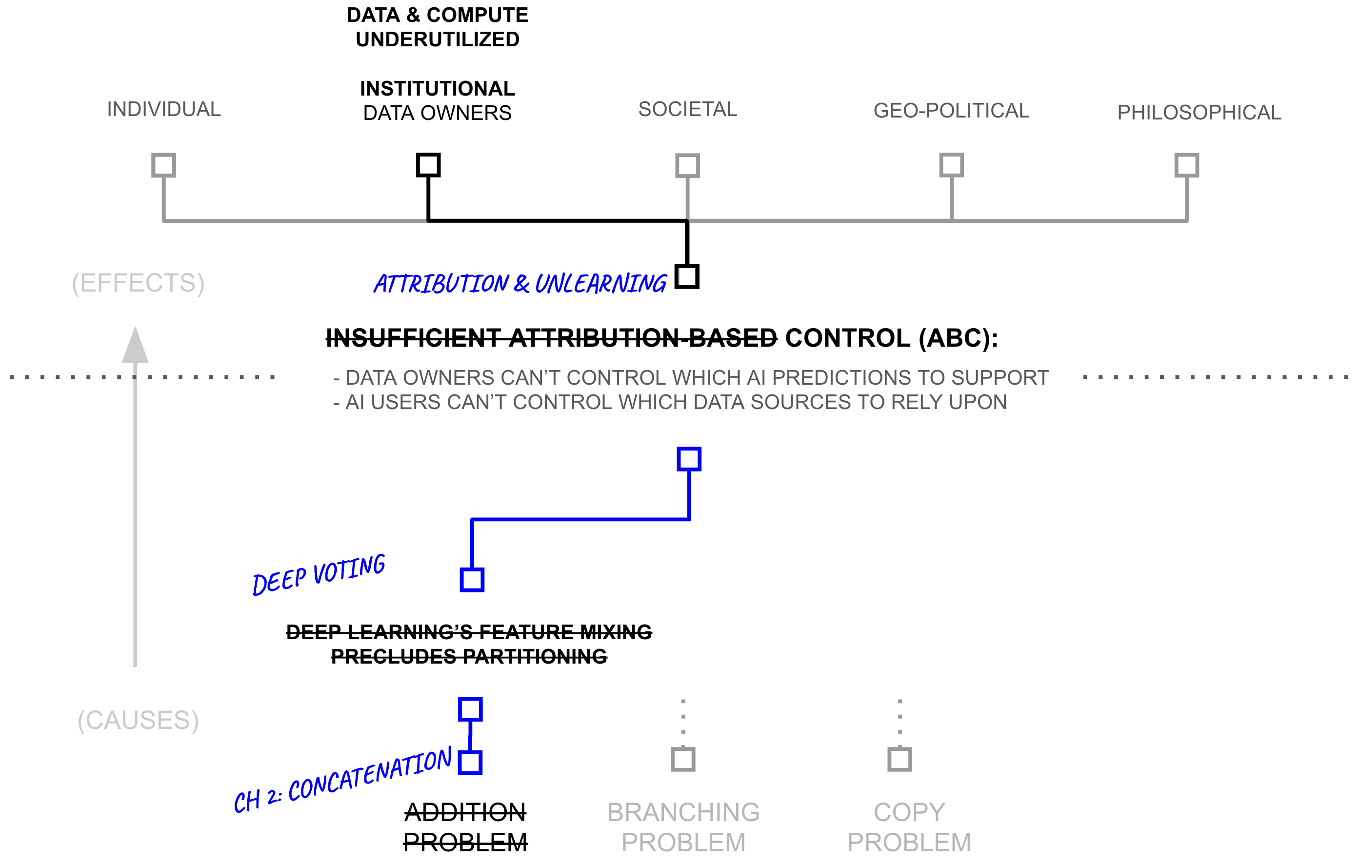
Current systems tend to choose a fixed point on this spectrum, making an explicit tradeoff between these competing forces. Deep voting formalizes a more continuous alternative: dynamic adjustment of these parameters (perhaps based on empirical information). When data shows high redundancy across sources (like common language patterns), higher λ values enable efficient parameter sharing. When sources contain unique information (like proprietary research), lower values maintain clearer attribution and better reward data owners for their novelty and innovation.
The empirical evidence presented earlier in this chapter paints a stark picture of current limitations. AI systems today access less than one millionth of the world’s digital data, 180 zettabytes versus roughly 180 terabytes for the largest known training sets. Even the largest AI firms utilize less than 5.57% of available compute capacity. Meanwhile, techniques like RETRO/ATLAS have demonstrated 25-50x parameter efficiency gains while maintaining performance, recent compression research shows 5-10x reduction in parameter counts without accuracy loss, and catastrophic forgetting work suggests a 40x drop in model size is attainable.
This tension yields our central empirical question: Can deep voting meaningfully shift the Pareto frontier between learning power, attribution clarity, and computational efficiency? Success could mean unlocking orders of magnitude more training data through clear attribution mechanisms. Success would enable dramatic reductions in computational waste through dynamic parameter sharing. Perhaps most importantly, success would create a path toward safe compute sharing through reliable influence tracking; the sparse, concatenated section could be distributed across multiple computers.
The stakes are significant. If deep voting succeeds, it could unlock another 6+ orders of magnitude of training data and compute productivity. If it fails, we may remain constrained by the fundamental limitations of current architectures. The next section examines the empirical evidence, providing an early view of whether deep voting might achieve the theoretical benefits suggested by its mathematical framework.
Empirical Evidence: Does the Pareto-Tradeoff Move?
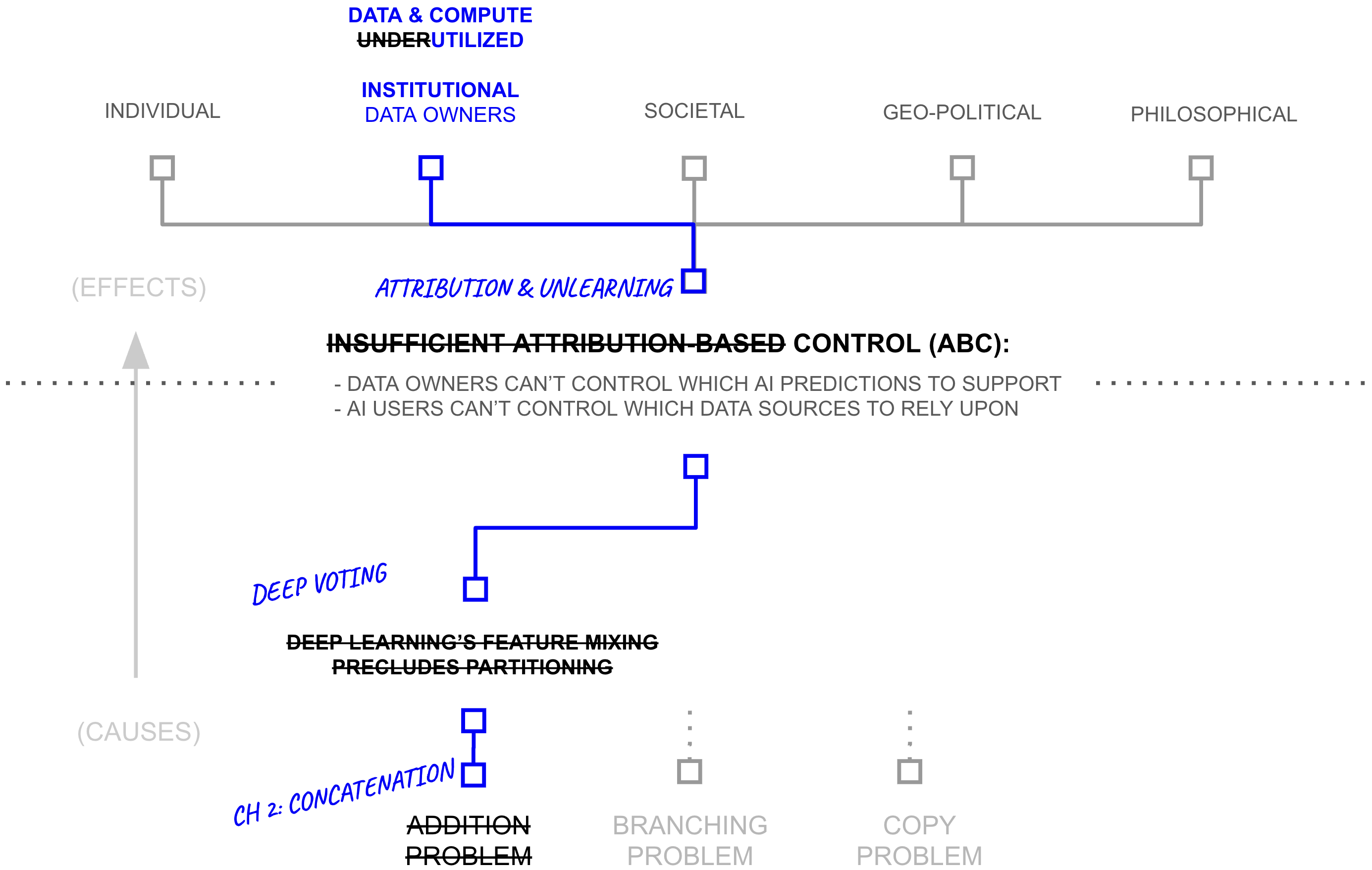
To evaluate whether deep voting can shift the fundamental tradeoffs between capability and attribution, we must first establish clear empirical baselines. Deep learning’s conventional wisdom around end-to-end training suggests a stark choice: systems can either achieve state-ofthe-art performance through dense feature mixing or maintain clear attribution, but not both. Yet recent results challenge this assumption. Consider the performance comparison between GPT-3 and RETRO, as described in Table 2.7 below.
The result demands explanation. RETRO matches GPT-3’s performance while using 25x fewer parameters and maintaining clear paths for attribution through its retrieval mechanism. If the tradeoffs between attribution and capability were truly fundamental, such a result should not be possible.
Pure Architectures: The Baseline Tradeoff
Conventional architectures exhibit clear tradeoffs between attribution, efficiency, and performance. We examine three points on this spectrum:
Traditional deep learning systems (λ = 1) achieve state-of-the-art performance through unrestricted parameter sharing. On MNIST, non-private models reach 98.3% accuracy, while an identically parameterized model with differential privacy constraints drops to 90% (Abadi et al., 2016). This performance advantage comes at a cost: unrestricted parameter mixing during training erases mappings between sources and predictions, making attribution impossible.
Group-based federated systems (λ = 0, γ = 1) maintain clear attribution boundaries by partitioning data within institutional silos. When data is independently and identically distributed (IID) across clients, this partitioning incurs no performance cost. However, when data is non-IID
| Subset | 7B Baseline (Ours) | GPT-3 | Jurassic-1 | Gopher | 7.5B |
|---|---|---|---|---|---|
| arxiv | 0.742 | 0.838 | 0.680 | 0.641 | 0.714 |
| books3 | 0.792 | 0.802 | 0.835 | 0.706 | 0.653 |
| dm_mathematics | 1.177 | 1.371 | 1.037 | 1.135 | 1.164 |
| freelaw | 0.576 | 0.612 | 0.514 | 0.506 | 0.499 |
| github | 0.420 | 0.645 | 0.358 | 0.367 | 0.199 |
| gutenberg_pg_19 | 0.803 | 1.163 | 0.890 | 0.652 | 0.400 |
| hackernews | 0.971 | 0.975 | 0.869 | 0.888 | 0.860 |
| nih_exporter | 0.650 | 0.612 | 0.590 | 0.590 | 0.635 |
| opensubtitles | 0.974 | 0.932 | 0.879 | 0.894 | 0.930 |
| philpapers | 0.760 | 0.723 | 0.742 | 0.682 | 0.699 |
| pile_cc | 0.771 | 0.698 | 0.669 | 0.688 | 0.626 |
| pubmed_abstracts | 0.639 | 0.625 | 0.587 | 0.578 | 0.542 |
| pubmed_central | 0.588 | 0.690 | 0.579 | 0.512 | 0.419 |
| stackexchange | 0.714 | 0.773 | 0.655 | 0.638 | 0.624 |
| ubuntu_irc | 1.200 | 0.946 | 0.857 | 1.081 | 1.178 |
| uspto_backgrounds | 0.603 | 0.566 | 0.537 | 0.545 | 0.583 |
| Average | 0.774 | 0.811 | 0.705 | 0.694 | 0.670 |
across clients, MNIST accuracy drops from 98.69% to 96.29% (Zhao et al., 2018)—a 2.4% degradation relative to joint training. This reflects a tension between attribution boundaries and cross-source pattern learning.
Pure memory-based approaches (λ = 0,γ = 0) such as k-NN provide perfect attribution by directly linking predictions to source examples. These systems achieve 97.2% accuracy on MNIST (Grover and Toghi 2018) but cannot generalize beyond patterns explicitly present in their memory banks.
These results establish baseline tradeoffs: dense architectures sacrifice attribution for performance, and federated/memory-based architectures sacrifice performance (on non-IID data) but gain attribution. The six orders of magnitude of inaccessible data and underutilized compute identified earlier remain siloed behind institutional boundaries because organizations cannot share data without relinquishing control. If these tradeoffs reflect fundamental constraints rather than architectural limitations, they would permanently restrict AI systems’ access to real-world resources
The First Crack: RETRO and ATLAS
However, recent architectures challenge these baseline tradeoffs. RETRO outperforms GPT-3 on the Pile (0.670 vs 0.811 bits-per-byte) while using only 7.5B parameters compared to GPT-3’s 175B. This constitutes a 25x reduction in parameter count while achieving superior performance and maintaining clear attribution paths through its retrieval mechanism (Borgeaud et al., 2022).
ATLAS demonstrates similar gains: 25-50x parameter efficiency improvements while maintaining or exceeding baseline performance (Izacard et al., 2023). Both systems achieve these results through a fundamental architectural shift: rather than compressing all knowledge into dense parameters, they maintain explicit connections to source documents through retrieval.
These results demonstrate that the tradeoff between attribution and capability reflects architectural choices rather than fundamental machine learning constraints. Systems maintaining explicit source separation through retrieval mechanisms achieve competitive performance with dense models while preserving attribution.
Converging Evidence Across Architectures
RETRO and ATLAS represent a broader pattern. Multiple architectural innovations demonstrate that explicit information paths enable simultaneous optimization of attribution and performance.
PATE (Private Aggregation of Teacher Ensembles) demonstrates this pattern in privacypreserving machine learning. Traditional privacy-preserving approaches incur 10-20% performance degradation. PATE reduces this gap to 0.7% on MNIST (98.5% accuracy versus 99.2% non-private baseline) while maintaining differential privacy guarantees through source-separated teacher ensembles (Papernot et al., 2018).
Federated RAG systems demonstrate concurrent improvements in attribution and performance. Recent work shows that federated RAG improves both attribution clarity and model accuracy simultaneously (Table 2.8) (Hou and Wang 2024).
| Task | Federated RAG Accuracy (%) | Baseline RAG Accuracy (%) |
|---|---|---|
| Task 1 | 78 | 70 |
| Task 2 | 82 | 75 |
| Task 3 | 74 | 68 |
| Task 4 | 88 | 80 |
| Task 5 | 81 | 76 |
Git Re-Basin demonstrates that independently trained models can be merged with minimal performance loss through weight permutation alignment (Ainsworth et al., 2022). This extends previous model merging results (Zhao et al., 2018) by enabling merging across models trained on separate dataset partitions from similar distributions. The technique identifies and corrects for arbitrary permutations of hidden layer neurons that occur during independent training, effectively aligning equivalent features across models before merging.
Deep Voting: Formalizing the Pattern
These architectures (RETRO, ATLAS, PATE, federated RAG, and Git Re-Basin) share a common technical mechanism: they replace addition operations during training with concatenation, deferring synthesis until inference time. We formalize this pattern as deep voting.
Traditional deep learning architectures synthesize knowledge during training by adding gradient updates into shared parameters. This pre-synthesis creates the documented tradeoffs: compressed representations lose attribution, strict partitioning loses cross-source patterns, and explicit storage loses efficiency. Deep voting defers this synthesis. Source-specific knowledge remains concatenated (partitioned) during training. At inference time, relevant partitions are selectively synthesized through weighted addition, with synthesis scope bounded by intelligence budgets (Section 2.7).
This architectural choice enables three simultaneous optimizations that conventional architectures trade off:
Attribution through source partitioning. Concatenated representations preserve source identity. RETRO and ATLAS maintain explicit mappings to source documents, enabling the source-level control required to unlock 6+ orders of magnitude of inaccessible data.
Efficiency through selective synthesis. Inference-time synthesis activates only relevant partitions. RETRO’s 25x parameter reduction and PATE’s 0.7% privacy-performance gap demonstrate that selective synthesis substantially reduces computational requirements.
Performance through shared computation. Shared syntactic components learn crosssource patterns without full parameter mixing. Git Re-Basin’s successful merging and federated RAG’s accuracy improvements demonstrate that partitioned training with shared components achieves competitive performance, avoiding the 2.4% degradation of pure federated approaches on non-IID data.
The convergent results across these architectures (operating in different domains with different implementations e.g. language modeling, privacy preservation, retrieval, model merging) indicate that this mechanism represents a fundamental alternative to dense parameter mixing rather than domain-specific engineering. Deep voting shifts the Pareto frontier between attribution, efficiency, and performance by preserving source mappings that addition destroys
These systems demonstrate that the architecture of deferred synthesis is sound. Whether it remains sound when assets are independently owned, when per-source privacy guarantees impose real constraints on how predictions are synthesized, requires a setting where these constraints actually bind. The next section explores an approximation of that scenario.
Empirical Prototype: Private Ensemble Aggregation with Intelligence Budgets
In this prototype, five frontier language models, each trained independently by a different organization on its own data and compute, are ensembled under a mechanism that enforces formal per-source influence bounds. The deep voting mechanism described above is instantiated in its simplest form through weighted voting: each model serves as a source-specific function \(g_s\), and the syntactic function \(f\) synthesizes their predictions at inference time. Differential privacy machinery (specifically, Rényi differential privacy Mironov, 2017 and the exponential mechanism McSherry and Talwar, 2007) implements the intelligence budget framework of Definition 2.7, yielding per-source influence bounds that operate in all three regimes (privacy, measurement, and attribution) simultaneously.
Experimental Setup
The prototype evaluates five frontier language models on a multiple-choice subset of the Humanity’s Last Exam (HLE) benchmark Phan et al., 2025. HLE is a dataset of 2,500 expert-crafted questions contributed by nearly 1,000 subject-matter experts across more than 500 institutions, spanning mathematics, physics, biology, chemistry, computer science, philosophy, and other domains. Approximately 76% of HLE questions require short exact-match answers; the remaining ~600 are multiple-choice. The evaluation is restricted to the 513 multiple-choice questions for which all five models produced valid responses, as the one-hot prediction format required by the weighted voting mechanism (Equation \(\eqref{eq:weighted_votes}\)) naturally applies to discrete choice among labeled alternatives.5 Each model is queried through the OpenRouter API, and its predicted answer is recorded as a one-hot vector \(p_s \in \{0,1\}^{C_q}\) for each question \(q\) with cardinality \(C_q\) (the number of answer choices). The models and their individual accuracies are:
5 All code, model predictions, and experimental results are available at github.com/iamtrask/deepvoting.
| Model (Source \(s\)) | Correct | Accuracy |
|---|---|---|
| Gemini 3.1 Pro | 228 | 44.4% |
| Claude Opus 4 | 204 | 39.8% |
| Gemini 3.0 Pro | 188 | 36.6% |
| GPT-5 Pro | 155 | 30.2% |
| Kimi K2.5 | 152 | 29.6% |
Each model serves as a source-specific function \(g_s\) in the deep voting framework. The prediction vector \(p_{s,q} = g_s(x_q)\) represents model \(s\)’s one-hot prediction for question \(q\). The syntactic function \(f\) is implemented as weighted voting:
\begin{equation}\label{eq:weighted_votes} v_j(q) = \sum_{s \in \mathcal{S}} \gamma[s] \cdot p_{s,q,j}, \quad j = 1, \ldots, C_q \end{equation}where \(\gamma[s] \in [\gamma_{\min}[s], \gamma_{\max}[s]]\) is the intelligence budget for source \(s\), and the ensemble prediction is \(\hat{y}(q) = \arg\max_j v_j(q)\).
Baseline: Non-Private Hedge Ensembling
The central challenge of deep voting is choosing the weights \(\gamma[s]\). If we knew in advance which models would perform well on which questions, we could assign optimal weights from the start. But we do not have access to future outcomes, so the weights must be learned from experience as queries arrive. This is a classic online learning problem: at each round, the ensemble must commit to a weighting before observing the correct answer, then update its beliefs based on the outcome. The literature on online convex optimization provides algorithms with strong regret guarantees for exactly this setting (Freund and Schapire, 1997; Kalai and Vempala, 2005).
Before introducing privacy mechanisms, it is useful to establish the performance of non-private ensemble aggregation using the Hedge algorithm (multiplicative weights update) Freund and Schapire, 1997. Hedge maintains weights \(w_s^{(t)}\) for each model \(s\) at round \(t\), updating them multiplicatively based on observed losses:
\begin{equation}\label{eq:hedge_update} w_s^{(t+1)} = w_s^{(t)} \cdot (1 - \eta)^{\ell_s^{(t)}}, \quad \ell_s^{(t)} = \mathbf{1}[\hat{y}_s(q_t) \neq y^*(q_t)] \end{equation}where \(\eta = 0.1\) is the learning rate and \(\ell_s^{(t)}\) is the 0-1 loss of model \(s\) on question \(q_t\). With 513 online rounds, the Hedge ensemble achieves 50.29% accuracy (258/513), exceeding the best individual model (Gemini 3.1 Pro, 44.4%) by 5.9 percentage points. This establishes the accuracy ceiling for any private variant, and the central question becomes what accuracy cost, if any, formal intelligence budgeting guarantees impose.
Private Aggregation: The Two-Phase FTPL Mechanism
Releasing either the Hedge weights or the full vote counts \(v(q)\) at each round would leak information about individual models’ predictions. The goal is to implement the intelligence budgets: each source \(s\) contributes with bounded influence \(\gamma[s] \in [\gamma_{\min}[s], \gamma_{\max}[s]]\), and the per-source cost of participation is quantified by the differential attribution. To build this mechanism, the prototype draws on two core primitives: the exponential mechanism for weight selection, and the Gaussian Noisy Max (GNMax) mechanism for private output release (Papernot et al., 2018). The DP machinery provides the formal accounting that makes intelligence budgets verifiable: each source’s \(\epsilon\) is precisely the differential attribution cost of its participation.
Differential Privacy: Definitions and Intuition. The formal guarantees rest on differential privacy (DP), introduced by Dwork, McSherry, Nissim, and Smith.6
6 C. Dwork, F. McSherry, K. Nissim, and A. Smith, “Calibrating Noise to Sensitivity in Private Data Analysis,” Theory of Cryptography (TCC), 2006. The presentation here follows the standard textbook formulation: C. Dwork and A. Roth, The Algorithmic Foundations of Differential Privacy, 2014, Definition 3.1.
Differential Privacy
A randomized mechanism \(\mathcal{M}\) satisfies \((\epsilon, \delta)\)-differential privacy if, for all neighboring datasets \(D, D’\) differing in one record and all measurable sets \(S\) of outputs:
\[ \Pr[\mathcal{M}(D) \in S] \leq e^{\epsilon} \cdot \Pr[\mathcal{M}(D’) \in S] + \delta \]When \(\delta = 0\), the mechanism satisfies pure \(\epsilon\)-differential privacy.
The parameter \(\epsilon\) bounds how much any single record can affect the output distribution. An observer who sees the mechanism’s output cannot reliably determine whether any particular record was present in the input, because the output distributions with and without that record are nearly indistinguishable. Smaller \(\epsilon\) means stronger privacy; \(\epsilon = 0\) would mean the output reveals nothing about any individual record (although it may still release information which is consistently present in a sufficiently large number of records; e.g. “what causes cancer” but not “does patient X have cancer?”).
In the ensemble setting, “neighboring datasets” correspond to changing one model’s prediction on one question. The goal is to ensure that the ensemble’s published outputs (the predicted answers) do not reveal too much about any individual model’s contribution.
Phase 1: Weight Calibration via Follow the Perturbed Leader. The mechanism replaces Hedge with Follow the Perturbed Leader (FTPL) Kalai and Vempala, 2005, an online learning algorithm that selects actions by perturbing cumulative utilities with random noise. At each calibration round \(t\), a model is selected by:
\begin{equation}\label{eq:ftpl} m^* = \arg\max_{m \in \mathcal{S}} \left\{ -L_m^{(t)} + \frac{Z_m}{\eta} \right\}, \quad Z_m \overset{\text{i.i.d.}}{\sim} \text{Gumbel}(0,1) \end{equation}where \(L_m^{(t)} = \sum_{\tau=1}^{t} \ell_m^{(\tau)}\) is the cumulative loss of model \(m\) through round \(t\) and \(\eta > 0\) is the learning rate. Here \(\text{Gumbel}(0,1)\) denotes the standard Gumbel distribution with CDF \(F(z) = e^{-e^{-z}}\), sampled via the inverse CDF as \(Z = -\ln(-\ln(U))\) for \(U \sim \text{Uniform}(0,1)\).
Why Gumbel noise? The choice of Gumbel perturbations is not arbitrary. By the Gumbel-max trick,7 when each \(Z_m\) is an independent \(\text{Gumbel}(0,1)\) draw, the probability of selecting model \(m\) follows a Gibbs (softmax) distribution:
7 The Gumbel-max trick states that if \(Z_1, \ldots, Z_K \overset{\text{i.i.d.}}{\sim} \text{Gumbel}(0,1)\), then \(\arg\max_k \{a_k + Z_k / \eta\}\) samples from the categorical distribution with \(\Pr[k] \propto \exp(\eta \, a_k)\). This result traces to extreme value theory (E.J. Gumbel, 1954) and the theory of discrete choice (R.D. Luce, 1959).
This distribution concentrates probability mass on models with low cumulative loss (strong past performance), with \(\eta\) controlling the concentration: larger \(\eta\) produces sharper distributions that favor the current leader, while smaller \(\eta\) produces more uniform distributions.
The exponential mechanism connection. The distribution in Equation \(\eqref{eq:ftpl_gibbs}\) is precisely the exponential mechanism of McSherry and Talwar.8 The exponential mechanism selects an option with probability proportional to \(\exp(\epsilon \cdot u(D, r) / (2\Delta u))\), where \(u(D, r)\) is the utility of option \(r\) on dataset \(D\) and \(\Delta u\) is the sensitivity. In the FTPL setting:
8 F. McSherry and K. Talwar, “Mechanism Design via Differential Privacy,” FOCS, 2007, Theorem 6: the exponential mechanism preserves \((\epsilon, 0)\)-differential privacy. In the FTPL context, the utility function is \(u(D, m) = -L_m\), sensitivity is \(\Delta u = 1\), and the temperature \(1/\eta\) corresponds to \(2/\epsilon\). Solving gives \(\epsilon = 2\eta\).
- Utility: \(u(D, m) = -L_m\), assigning higher utility to models with lower cumulative loss.
- Sensitivity: \(\Delta u = 1\), because changing one question’s outcome changes one model’s cumulative loss by at most 1.
- Matching terms: FTPL selects \(m\) with probability \(\propto \exp(-\eta \cdot L_m) = \exp(\eta \cdot u(D,m))\). The exponential mechanism selects with probability \(\propto \exp(\epsilon \cdot u(D,m) / 2)\). Equating \(\eta = \epsilon / 2\) gives \(\epsilon = 2\eta\).
The Gumbel perturbation that FTPL adds for online learning (to explore alternatives and achieve low regret) turns out to be exactly the noise that differential privacy requires. There is no additional privacy cost beyond what the learning algorithm already uses. With \(\eta = 0.1\), each calibration round costs only \(\epsilon = 0.2\) in pure differential privacy.
To compute smooth ensemble weights rather than selecting a single model per round, the mechanism averages over \(N = 2{,}000\) independent Gumbel draws, obtaining \(\gamma[s] = \frac{1}{N} \sum_{i=1}^{N} \mathbf{1}[m^*_i = s]\). After \(T\) calibration questions, weights are frozen: \(\gamma_{\text{frozen}}[s] = \gamma[s]^{(T)}\). All subsequent computations using frozen weights incur no additional privacy cost from the FTPL mechanism, by the post-processing theorem of differential privacy.9
9 Dwork and Roth (2014), Proposition 2.1: any deterministic function of the output of an \((\epsilon, \delta)\)-DP mechanism is itself \((\epsilon, \delta)\)-DP. Since frozen weights are derived from the FTPL output, further computations on them inherit the same guarantee without additional cost.
Phase 2: Deployment via Confident-GNMax. During deployment (after calibration), the frozen weights define the ensemble. The remaining privacy question is how to release predictions without revealing too much about individual models’ votes. The Gaussian Noisy Max (GNMax) mechanism addresses this by releasing only the index of the highest noisy vote, rather than the full vote vector:
\begin{equation}\label{eq:gnmax} \hat{y}(q) = \arg\max_j \left\{ v_j(q) + \mathcal{N}(0, \sigma^2) \right\} \end{equation}where \(v_j(q)\) is the weighted vote count from Equation \(\eqref{eq:weighted_votes}\) and \(\sigma > 0\) controls the noise scale. To further reduce privacy expenditure on queries where the ensemble has low confidence, the prototype applies the Confident-GNMax thresholding mechanism (Papernot et al., 2018):
\begin{equation}\label{eq:confident_gnmax} \hat{y}(q) = \begin{cases} \arg\max_j \left\{ v_j(q) + \mathcal{N}(0, \sigma^2) \right\} & \text{if } \max_j v_j(q) + \mathcal{N}(0, \sigma^2) \geq \mathcal{T} \\ \bot & \text{otherwise} \end{cases} \end{equation}where \(\mathcal{T} \geq 0\) is the confidence threshold and \(\bot\) denotes refusal to answer. Refused queries contribute zero privacy cost: the system reveals only that the ensemble was not sufficiently confident, which (because the confidence check itself uses noisy counts) leaks minimal information about any individual model.
Privacy Accounting via Rényi Differential Privacy. The full mechanism involves multiple private operations: \(T\) rounds of FTPL weight selection (each satisfying \(0.2\)-DP) and up to \(Q\) rounds of GNMax during deployment. Rényi differential privacy (RDP) provides substantially tighter composition by tracking privacy loss through Rényi divergences, a family of information-theoretic measures parameterized by an order \(\alpha > 1\).10
10 I. Mironov, “Rényi Differential Privacy,” IEEE CSF, 2017. RDP composes additively at each order \(\alpha\) (Proposition 1), and converts to standard \((\epsilon, \delta)\)-DP by optimizing over \(\alpha\) (Proposition 3).
Rényi Differential Privacy
A randomized mechanism \(\mathcal{M}\) satisfies \((\alpha, \hat{\epsilon})\)-RDP if for all neighboring datasets \(D, D’\):
\[ D_\alpha(\mathcal{M}(D) \| \mathcal{M}(D’)) = \frac{1}{\alpha - 1} \log \mathbb{E}\left[ \left( \frac{\Pr[\mathcal{M}(D) = o]}{\Pr[\mathcal{M}(D’) = o]} \right)^\alpha \right] \leq \hat{\epsilon} \]where \(D_\alpha(\cdot \| \cdot)\) denotes the Rényi divergence of order \(\alpha > 1\) (Mironov, 2017).
While standard DP bounds the worst-case multiplicative change in output probabilities (by \(e^{\epsilon}\)), RDP bounds a soft average of these changes, parameterized by \(\alpha\). The practical advantage of tracking RDP at multiple orders simultaneously is that composition remains additive: if mechanism \(\mathcal{M}_1\) satisfies \((\alpha, \epsilon_1)\)-RDP and \(\mathcal{M}_2\) satisfies \((\alpha, \epsilon_2)\)-RDP, their sequential composition satisfies \((\alpha, \epsilon_1 + \epsilon_2)\)-RDP.
Data-dependent GNMax bound. For the GNMax mechanism, the RDP cost per query depends on the margin between the top two vote counts. Let \(\Delta(q) = v_{(1)}(q) - v_{(2)}(q)\) be this margin. The \((\alpha, \hat{\epsilon}_\alpha(q))\)-RDP cost satisfies:11
11 Papernot et al. (2018), Theorem 6: the data-dependent RDP bound exploits the vote margin. When the plurality vote has a large margin, the Gaussian noise is unlikely to change the outcome, so privacy cost decreases exponentially with the squared margin.
The practical consequence is that when the ensemble strongly agrees (\(\Delta(q)\) large relative to \(\sigma\)), the privacy cost per query decreases exponentially with the squared margin. In a well-calibrated ensemble where the majority of queries have large margins, most deployment queries contribute near-zero privacy cost.
Full composition. The total system RDP across \(T\) calibration rounds and the answered deployment queries composes additively at each order \(\alpha\):
\begin{equation}\label{eq:rdp_composition} \hat{\epsilon}_\alpha^{\text{total}} = \underbrace{\sum_{t=1}^{T} \left[ \hat{\epsilon}_\alpha^{\text{GNMax}}(q_t) + \epsilon_{\text{FTPL}} \right]}_{\text{Phase 1: calibration}} + \underbrace{\sum_{q \in \mathcal{Q}_{\text{answered}}} \hat{\epsilon}_\alpha^{\text{GNMax}}(q)}_{\text{Phase 2: deployment}} \end{equation}The final \((\epsilon, \delta)\)-DP guarantee is obtained by converting the composed RDP bound to standard differential privacy, optimizing over the Rényi order \(\alpha\):
\begin{equation}\label{eq:rdp_to_dp} \epsilon = \min_{\alpha > 1} \left\{ \hat{\epsilon}_\alpha^{\text{total}} + \frac{\ln(1/\delta)}{\alpha - 1} \right\} \end{equation}The prototype evaluates this expression at 13 values of \(\alpha \in \{1.5, 2, 3, 4, 5, 8, 10, 16, 20, 32, 50, 64, 100\}\) and reports the minimum.
Individual Intelligence Budgets: Per-Source Privacy Accounting
The mechanism above provides a system-level privacy guarantee. To implement intelligence budgets, this section extends it to per-source privacy accounting that controls each model’s individual influence on the ensemble output.
Per-Source Sensitivity
In the weighted voting mechanism of Equation \(\eqref{eq:weighted_votes}\) with one-hot predictions \(p_s \in \{0,1\}^{C_q}\), the \(\ell_2\)-sensitivity of the vote vector \(v(q)\) to source \(s\)’s prediction is:
\[ \Delta_s = \gamma[s] \cdot \sqrt{2} \]Proof. If source \(s\) changes its prediction from one-hot vector \(e_j\) to \(e_k\) (\(j \neq k\)), the vote vector changes by \(\gamma[s] \cdot (e_k - e_j)\), which has \(\ell_2\)-norm \(\gamma[s] \cdot \sqrt{1^2 + 1^2} = \gamma[s]\sqrt{2}\).
Under the Gaussian mechanism with noise \(\mathcal{N}(0, \sigma^2 I)\), the standard RDP bound for \(\ell_2\)-sensitivity \(\Delta_s\) gives the per-source RDP cost at order \(\alpha\):
\begin{equation}\label{eq:per_source_rdp} \hat{\epsilon}_\alpha^{(s)}(q) = \frac{\alpha \cdot \Delta_s^2}{2\sigma^2} = \frac{\alpha \cdot \gamma[s]^2}{\sigma^2} \end{equation}The intelligence budget \(\gamma[s]\) therefore directly controls the per-query privacy cost. The weight \(\gamma[s]\) simultaneously determines how much source \(s\) contributes to the prediction (the attribution semantics) and how much privacy source \(s\) expends (the privacy semantics), which is exactly the coupling that attribution-based control requires. The relationship is quadratic: doubling a source’s influence quadruples its per-query privacy cost.
Individual Intelligence Budget Mechanism
For each source \(s \in \mathcal{S}\), define:
- \(\gamma_{\min}[s] > 0\): minimum weight (attribution floor, ensuring source \(s\) always has at least this much influence)
- \(\gamma_{\max}[s] \leq 1\): maximum weight (privacy ceiling, ensuring source \(s\) never exceeds this influence)
- \(B(s) > 0\): total privacy budget (cumulative \(\epsilon\) limit over all queries)
The per-query spend for source \(s\) at query \(q\) is \(\hat{\epsilon}_\alpha^{(s)}(q) = \alpha \cdot \gamma[s]^2 / \sigma^2\). The cumulative spend must satisfy:
\[ \sum_{q=1}^{Q} \hat{\epsilon}_\alpha^{(s)}(q) \leq B(s) \]When source \(s\) exhausts its budget, its weight collapses to \(\gamma_{\min}[s]\) and remaining sources’ weights are renormalized.
This mechanism exhibits all three ABC regimes simultaneously across different sources within the same ensemble:
- Privacy regime (\(\gamma_{\max}[s]\) small, \(B(s)\) tight): Source \(s\) has minimal influence per query and may exhaust its budget, collapsing to \(\gamma_{\min}[s]\). This provides strong privacy guarantees.
- Measurement regime (\(\gamma_{\max}[s]\) moderate, \(B(s)\) moderate): Source \(s\) contributes meaningfully but with tracked spend. The system can report exactly how much influence source \(s\) had on each prediction.
- Attribution regime (\(\gamma_{\max}[s]\) large, \(B(s)\) generous): Source \(s\) dominates the ensemble while its influence remains bounded and auditable.
Experimental Results
Per-Source Privacy–Accuracy Tradeoff. All privacy costs below are reported per source: the \(\epsilon\) that each data owner pays for participating in the ensemble, not a system-wide total. This is the metric that matters for a data owner deciding whether to contribute.
A sweep across four ensemble sizes (top-2 through top-5 models by individual accuracy), calibration lengths \(T \in \{10, 25, 50, 75, 100, 200\}\), noise scales \(\sigma \in \{1, 2, 5, 10, 20\}\), and confidence thresholds \(\mathcal{T} \in \{0.0, 0.15, 0.30, 0.50\}\) produces 480 configurations.
| Ensemble | \(T\) | \(\sigma\) | Accuracy | \(\epsilon_{\max}\) | \(\epsilon_{\min}\) | Hedge |
|---|---|---|---|---|---|---|
| Top-2 | 10 | 20 | 51.07% | 4.3 | 3.7 | 51.07% |
| Top-3 | 10 | 20 | 48.73% | 3.4 | 2.5 | 51.27% |
| Top-3 | 50 | 20 | 51.27% | 8.4 | 6.2 | |
| Top-4 | 50 | 20 | 48.34% | 7.8 | 6.0 | 50.49% |
| Top-4 | 75 | 20 | 50.49% | 11.6 | 8.3 | |
| Top-5 | 25 | 20 | 45.42% | 4.4 | 3.5 | 50.29% |
| Top-5 | 75 | 20 | 48.15% | 11.1 | 8.2 | |
| Top-5 | 100 | 20 | 50.10% | 14.5 | 10.6 |
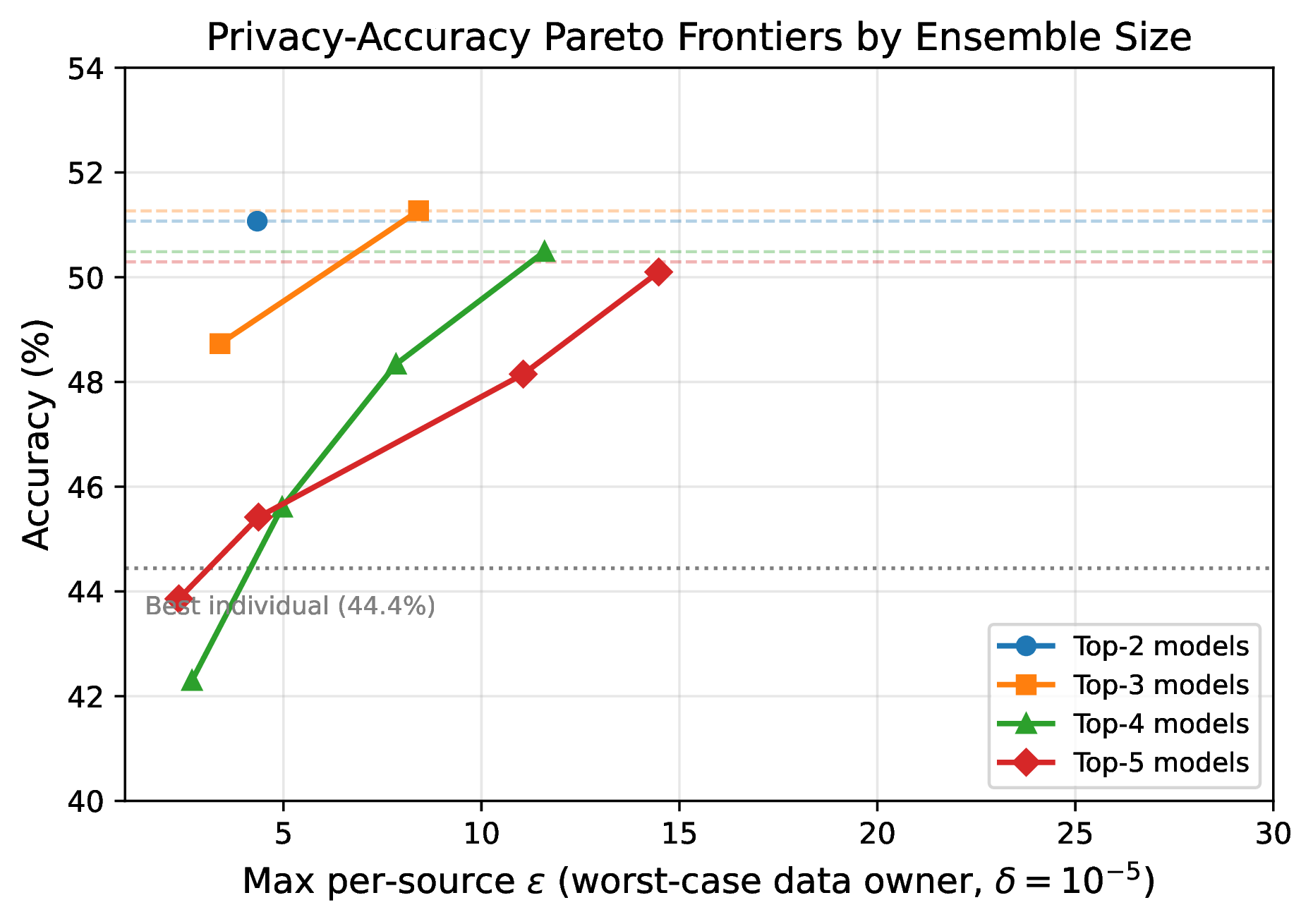
Three findings emerge. First, even the smallest ensemble (top-2) matches the non-private Hedge exactly (51.07%) at just \(\epsilon_{\max} = 4.3\) per source. Second, the per-source cost varies with weight: Gemini 3.1 Pro (the highest-weighted model) consistently pays the most, while lower-ranked models join at 15–30% lower cost. Third, a data owner can choose its operating point on the Pareto frontier: the top-3 ensemble beats the best individual model at \(\epsilon_{\max} = 3.4\) per source (+4.3pp accuracy gain), or matches the Hedge at \(\epsilon_{\max} = 8.4\).
Coverage Tradeoff. The Confident-GNMax threshold \(\mathcal{T}\) controls a coverage–privacy tradeoff: by refusing to answer queries where the ensemble lacks consensus, the mechanism reduces privacy spend while improving accuracy on answered queries.
| \(\mathcal{T}\) | Coverage | \(\epsilon_{\max}\) | Acc. (answered) | (\(T\), \(\sigma\)) |
|---|---|---|---|---|
| 0.00 | 100% | 2.4 | 43.86% | (10, 20) |
| 0.15 | 54% | 2.0 | 45.85% | (10, 20) |
| 0.50 | 53% | 2.0 | 45.42% | (10, 20) |
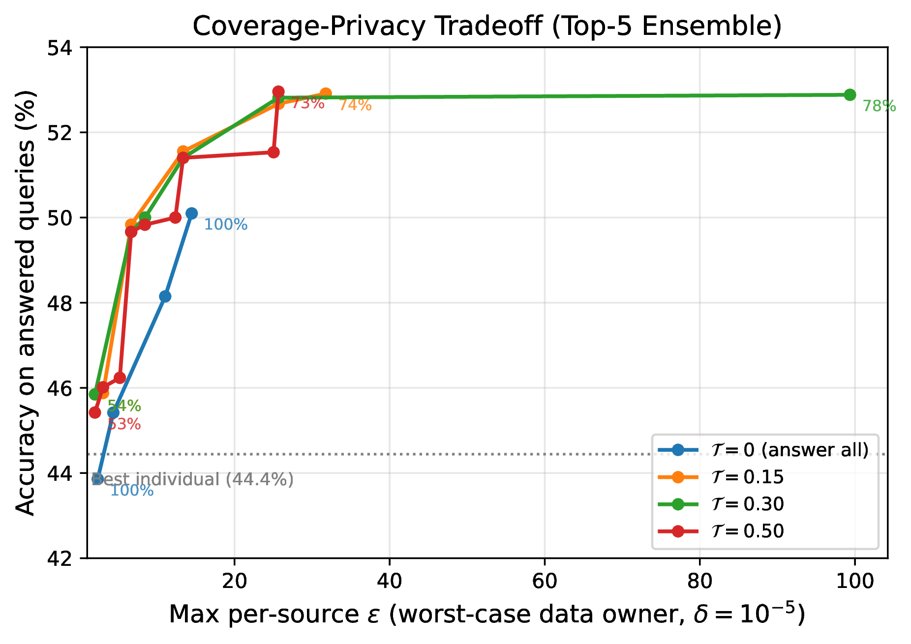
Per-Source Cost Structure. The pattern is consistent: privacy cost tracks influence. The highest-weighted model (Gemini 3.1 Pro) always pays the most, while each additional lower-ranked model joins at progressively lower cost. This is the mechanism working as designed: a source that contributes more influence expends more of its privacy budget, and a source seeking minimal privacy exposure can participate with a low weight and pay commensurately less.
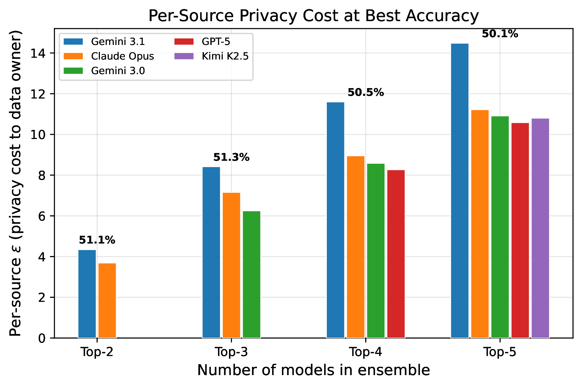
This cost structure has a natural economic interpretation. The per-source \(\epsilon\) is effectively the price a data owner pays for a given level of influence over predictions. A data owner deciding whether to contribute its model to an ensemble can choose where on this tradeoff to sit: higher weight buys more influence (and thus more credit, compensation, or attribution) at the cost of more privacy exposure, while lower weight preserves privacy at the cost of reduced influence.
Individual Budget Demonstration. To demonstrate the intelligence budget mechanism, heterogeneous budgets are assigned reflecting diverse stakeholder preferences:
| Model | \(\gamma_{\min}\) | \(\gamma_{\max}\) | \(B(s)\) | \(\hat{\epsilon}\)/query | Max Qs | Regime |
|---|---|---|---|---|---|---|
| Gemini 3.1 Pro | 0.10 | 0.60 | 100.0 | 0.720 | 138 | Attribution |
| Claude Opus 4 | 0.08 | 0.40 | 40.0 | 0.320 | 125 | Measurement |
| Gemini 3.0 Pro | 0.05 | 0.35 | 30.0 | 0.245 | 122 | Measurement |
| GPT-5 Pro | 0.03 | 0.20 | 10.0 | 0.080 | 125 | Privacy |
| Kimi K2.5 | 0.02 | 0.15 | 5.0 | 0.045 | 111 | Privacy |
With \(T = 100\) calibration questions and \(\sigma = 1.0\), the individual DP mechanism produces the following dynamics:
- Calibration (Q1–Q100): FTPL learns optimal weights within each model’s \([\gamma_{\min}, \gamma_{\max}]\) band. Gemini 3.1 Pro quickly rises to its ceiling (\(\gamma \approx 0.63\) after normalization), reflecting its superior accuracy. Lower-performing models settle near their floors.
- Budget exhaustion (Q100–Q300): Models with tight budgets progressively exhaust their spend. Kimi K2.5 exhausts at Q149 (spent 5.0/5.0), collapsing to \(\gamma_{\min} = 0.02\). Gemini 3.1 Pro, despite having the largest budget, exhausts at Q186 because its high weight (\(\gamma \approx 0.63\)) costs \(0.79\epsilon\) per query.
- Graceful degradation: As each model collapses to \(\gamma_{\min}\), remaining active models’ weights increase through renormalization. Rather than failing catastrophically, the ensemble smoothly transitions from optimal weighting toward more uniform weighting as budgets deplete.
The ensemble achieves 49.12% accuracy under these individual constraints, only 1.17 percentage points below the unconstrained Hedge, while providing per-source influence guarantees that no source exceeds its allocated budget.
Discussion
The constraints bind, and the architecture holds. Combining independently trained AI assets under formal per-source influence control produces an ensemble that exceeds the accuracy of every individual contributor, at a per-source privacy cost that is moderate and transparent.
Dual-purpose noise. FTPL’s Gumbel perturbation simultaneously provides regret-minimizing exploration (Kalai and Vempala, 2005) and \(\epsilon\)-differential privacy (McSherry and Talwar, 2007), avoiding the typical cost of adding privacy to online learning algorithms. This duality reflects a deeper alignment between the information-theoretic requirements of exploration and privacy: both require that the mechanism’s output cannot be too sensitive to any single data point.
Data-dependent accounting. The GNMax RDP bound ensures that high-consensus queries (which predominate when the ensemble is well-calibrated) cost exponentially less than worst-case bounds predict. In these experiments, the majority of deployment queries have near-zero RDP cost because the ensemble’s margin \(\Delta(q)\) is large relative to \(\sigma\).
Influence bands. The \([\gamma_{\min}, \gamma_{\max}]\) mechanism provides simultaneous upper and lower bounds on each source’s influence, implementing ABC’s core requirement of per-source control. The lower bound \(\gamma_{\min}\) guarantees attribution; the upper bound \(\gamma_{\max}\) constrains privacy exposure; and the budget \(B(s)\) limits total cumulative influence over time.
Scaling considerations. The prototype is limited by its small ensemble size (\(|\mathcal{S}| = 5\)). In the PATE literature (Papernot et al., 2018), per-source costs decrease further as the number of teachers grows, because margins \(\Delta(q)\) increase with more agreeing voters while the sensitivity per teacher decreases. With hundreds of model slices, per-query costs would decrease by orders of magnitude, enabling per-source budgets of \(\epsilon < 1\) while answering thousands of queries.
Connection to the deep voting thesis. Each of the five models in this prototype was trained independently on its own data, using its own compute infrastructure. Ensembling them is, in effect, combining their data and compute. The private ensemble achieves 50.1–51.3% accuracy on HLE’s multiple-choice subset, surpassing all five constituent models. At the per-source level, this accuracy gain costs the worst-case data owner \(\epsilon = 4.3\) (top-2 ensemble) to \(\epsilon = 14.5\) (top-5 ensemble).
These five models were trained on substantially overlapping subsets of publicly available internet data, and they represent a vanishingly small fraction of the 6+ orders of magnitude of siloed data and underutilized compute documented in Section 2.2. The fact that ensembling even five models with overlapping training data already yields a +5.9 percentage point accuracy gain over the best individual model, while respecting per-source privacy bounds, suggests that the returns from accessing genuinely diverse, non-overlapping data through these budgeting mechanisms would be substantially greater.
From differential privacy to intelligence budgets. The per-source \(\epsilon\) values reported throughout this section are not merely privacy parameters. They are the differential attribution costs, measured on the actual dataset: each source’s \(\epsilon_s\) quantifies how much the ensemble’s output distribution changes when that source is included versus excluded. This is the intelligence budget framework made concrete. A data owner considering whether to contribute a model to a deep voting ensemble can inspect these bounds in advance, calibrate the influence they are willing to spend, and verify after the fact that the mechanism honored the contract.
Deep Voting: A Path to 6+ Orders of Magnitude
Deep voting addresses the addition problem that blocks access to 6+ orders of magnitude of data and compute. By preserving source attribution through concatenated representations while enabling cross-source learning through shared components, deep voting architectures demonstrate that the baseline tradeoffs between attribution, efficiency, and performance reflect architectural choices rather than fundamental constraints. Empirically, RETRO and ATLAS achieve 25–50x parameter efficiency while maintaining performance. PATE reduces privacy-performance gaps from 10–20% to 0.7%. Git Re-Basin enables merging of independently trained models. Federated RAG improves both attribution and accuracy simultaneously. These systems operate at scale today, processing real workloads with working implementations.
The implications for data access are direct. Current LLM training sets use approximately 180TB of text data. Global digital data reaches 180 zettabytes (6–9 orders of magnitude larger). Vast institutional repositories remain inaccessible primarily due to attribution and control concerns (Youssef et al., 2023). Deep voting’s source-partitioned architecture provides the attribution mechanism these institutions require, establishing a viable technical path to unlock this siloed data. Similarly, the implications for compute efficiency are substantial. The 6+ orders of magnitude of training inefficiency documented in Section 2.2.1 stems from retraining overhead, dense forward propagation, parameter redundancy, and catastrophic forgetting. Deep voting’s deferred synthesis architecture addresses each source: partitioned training enables selective retraining, inference-time synthesis enables sparse activation, source separation reduces redundancy, and explicit organization prevents catastrophic forgetting.
Deep voting addresses the addition problem. Source-partitioned representations preserve attribution. Deferred synthesis enables efficiency. Shared components enable performance. The architecture has been demonstrated at scale across multiple systems and domains.
The empirical prototype in the preceding section offers a concrete illustration of these dynamics. Five frontier language models, each trained independently by a different organization on its own data and compute, were ensembled under a mechanism that enforces per-source influence bounds through individual differential privacy budgets. The resulting ensemble exceeded the accuracy of every constituent model on the HLE benchmark by up to 6.9 percentage points, with per-source privacy costs of \(\epsilon = 3\)–\(15\) depending on influence level. The overhead imposed by influence management was measurably smaller than the accuracy gained from aggregation.
The prototype operates at the very bottom of the scaling curve. These five models were trained on overlapping subsets of publicly available data, collectively representing a tiny fraction of the resources documented in Section 2.2: the 6+ orders of magnitude of siloed training data (180 zettabytes vs. the ~180 TB consumed by current frontier models) and the orders-of-magnitude compute inefficiency from retraining, dense propagation, and catastrophic forgetting. If formal influence control over five sources with largely overlapping data already yields a considerable accuracy gain (+5.9pp even under per-source privacy constraints), the potential gains from hundreds or thousands of genuinely diverse sources (medical records, proprietary research, institutional archives, specialized sensor data), drawing on these 6+ orders of magnitude of untapped resources, would be far greater.
The per-source cost structure also has a direct economic implication. Because each source’s privacy cost is proportional to its influence weight, the intelligence budget mechanism creates a natural market in which data owners can calibrate across many ensembles how much influence they wish to contribute, treating their privacy budget as a resource to be allocated strategically. The fact that each source can see exactly what participation costs is precisely the kind of guarantee that would enable the institutional data holders documented in Section 2.2 to participate where they currently cannot.
However, solving the addition problem reveals a deeper challenge: the copy problem. Even if one achieved perfect attribution through deep voting, data sources cannot enforce how their contributions are used because whoever possesses a copy of the model retains unilateral control. Chapter 3 addresses this challenge, introducing techniques that enable attribution-based control rather than mere attribution-based suggestions.
References
- (2020). Scaling Laws for Neural Language Models. arXiv:2001.08361.
- (2022). Training Compute-Optimal Large Language Models. arXiv:2203.15556.
- (2024). OpenAI cofounder Ilya Sutskever says the way AI is built is about to change. The Verge.
- (2022). Improving language models by retrieving from trillions of tokens. ICML 2022, 2206–2240.
- (2023). Atlas: Few-shot Learning with Retrieval Augmented Language Models. Journal of Machine Learning Research, 24, 1–43.
- (2023). Towards lossless dataset distillation via difficulty-aligned trajectory matching. arXiv:2310.05773.
- (2016). Deep Learning. MIT Press.
- (2018). Measuring Catastrophic Forgetting in Neural Networks. AAAI 2018.
- (2024). How much LLM training data is there, in the limit? Educating Silicon.
- (2013). Building high-level features using large scale unsupervised learning. IEEE Transactions on Pattern Analysis and Machine Intelligence.
- (2012). ImageNet Classification with Deep Convolutional Neural Networks. NeurIPS 2012.
- (2014). Visualizing and Understanding Convolutional Networks. ECCV 2014.
- (2014). Aspects of the Theory of Syntax. MIT Press.
- (2006). Calibrating noise to sensitivity in private data analysis. TCC 2006.
- (2020). Individual Privacy Accounting via a Renyi Filter. arXiv:2008.11193.
- (2018). Scalable Private Learning with PATE. ICLR 2018.
- (2018). Federated Learning with Non-IID Data. arXiv:1806.00582.
- (2022). Git Re-Basin: Merging Models modulo Permutation Symmetries. arXiv:2209.04836.
- (2024). A Survey of Machine Unlearning. arXiv:2209.02299.
- Ml training with cloud gpu shortages: Is cross-region the answer? In Proceedings of the 4th Workshop on Machine Learning and Systems, EuroMLSys ’24, page 107–116, New York, NY, USA. Association for Computing Machinery.
- Nvidia hits new milestone as world’s first $5tn company, 10.
- Nvidia faces revenue threat from new u.s. ai chip export curbs, analysts say. Reuters, January. Updated January 13, 2025 6:31 PM GMT.
- There’s an ai war, and nvidia is the only arms dealer: Analyst. Yahoo Finance, May. Updated May 25, 2023.
- Most of openai’s 2024 compute went to experiments. Accessed: 2025-11-02.
- Deepseekmoe: Towards ultimate expert specialization in mixture-of-experts language models. arXiv preprint arXiv:2401.06066.
- Introducing llama 3.1: Our most capable models to date. Meta AI Blog, July. Published July 23, 2024.
- Language models are few-shot learners. arXiv preprint arXiv:2005.14165.
- Openai ceo sam altman says lack of compute capacity is delaying the company’s products. TechCrunch, October. Published 12:37 PM PDT, October 31, 2024.
- Data on ai models, 07. Accessed: 2025-11-02.
- Zuckerberg says Meta will need 10x more computing power to train Llama 4 than Llama 3. TechCrunch, aug. 12:53 AM PDT.
- Learning to reason with LLMs. sep. Introduces OpenAI o1, a new large language model trained with reinforcement learning for complex reasoning
- Training compute of frontier AI models grows by 4-5x per year. ´ Epoch AI Blog, may. Analysis of AI model compute trends showing 4-5x yearly growth from 2010 to 2024.
- Sweeps: An overview. Online tutorial for using W&B Sweeps for hyperparameter optimization.
- Llm surgery: Efficient knowledge unlearning and editing in large language models. arXiv preprint arXiv:2409.13054.
- Why there is no AI without inference. WSJ Partner Content sponsored by Arm, Vice President of Machine-Learning Technology.
- Overcoming catastrophic forgetting in neural networks. Proceedings of the National Academy of Sciences, 114(13):3521–3526.
- Data on machine learning hardware. Updated December 30, 2024
- Redpajama-data-v2: An open dataset with 30 trillion tokens for training large language models, 10. The dataset includes data processing tools for CommonCrawl data, focusing on five languages: English, French, Spanish, German, and Italian. It provides over 40 quality annotations for filtering and weighting data, including natural language indicators, repetitiveness measures, and content-based signals.
- Democracy of sound: Music piracy and the remaking of American copyright in the twentieth century. Oxford University Press.
- Common Crawl. Last edited on 30 December 2024, at 01:48 (UTC).
- A message from internet archive founder, brewster kahle. Internet Archive donation page detailing the organization’s mission, impact, and ways to support. The Archive hosts over 99 petabytes of data, including 625 billion webpages, 38 million texts, and 14 million audio recordings. Federal Tax ID: 94-3242767.
- Open source intelligence on the internet – categorisation and evaluation of search tools. Internal Security Review, 31:383–412.
- Amount of data created, consumed, and stored 2010-2023, with forecasts to 2028, 5. Accessed: December 31, 2024.
- Business facts: Essential business statistics you should know in 2025.
- The vanishing gradient problem during learning recurrent neural nets and problem solutions. International Journal of Uncertainty, Fuzziness and Knowledge-Based Systems, 6(02):107–116.
- Which neural net architectures give rise to exploding and vanishing gradients? Advances in neural information processing systems, 31.
- Individual differential privacy: A utility-preserving formulation of differential privacy guarantees. CoRR, abs/1612.02298.
- The algorithmic foundations of differential privacy. e, Foundations and Trends® in Theoretical Computer Science, 9(3–4):211–407.
- Jurassic-1: Technical details and evaluation. White Paper. AI21 Labs.
- Scaling language models: Methods, analysis & insights from training Gopher. arXiv preprint.
- Mnist dataset classification utilizing k-nn classifier with modified sliding-window metric. arXiv preprint arXiv:1809.06846.
- Large language model with federated retrieval-augmented generation for improved knowledge retrieval.
- Organizational factors in clinical data sharing for artificial intelligence in health care. JAMA Network Open, 6:e2348422, 12.
- (2016). Deep learning with differential privacy. Proceedings of the 2016 ACM SIGSAC Conference on Computer and Communications Security (CCS'16).
- (2024). Statistical guarantees for sparse deep learning. AStA Advances in Statistical Analysis, 108(2), 231–258.
- (2017). Rényi Differential Privacy. IEEE 30th Computer Security Foundations Symposium (CSF), 263–275.
- (2007). Mechanism Design via Differential Privacy. 48th Annual IEEE Symposium on Foundations of Computer Science (FOCS), 94–103.
- (2005). Efficient Algorithms for Online Decision Problems. Journal of Computer and System Sciences, 71(3), 291–307.
- (1997). A Decision-Theoretic Generalization of On-Line Learning and an Application to Boosting. Journal of Computer and System Sciences, 55(1), 119–139.
- (2025). Humanity's Last Exam. arXiv:2501.14249.